Evaluating Transferability and Validation Protocols of Convolutional Neural Networks for Acoustic Water Leak Detection Using SebaKMT Logger Recordings
Aleksandr Ivanaiskii, PhD
Industrial AI Founder & Systems Architect
Evgeny Ivanaiskii, PhD
Domain Expert
Sergei Shipilov
AI Architecture Lead, Rivixi LLC
Abstract
Limited labeled data from a newly deployed logger motivate training acoustic leak classifiers on recordings from other instruments. This study evaluates direct transfer, supervised target adaptation, and validation design using SebaKMT recordings. A single-scale convolutional neural network (CNN) with 25,633 parameters is compared with two three-branch networks containing 76,769 parameters and using repeated or distinct spectral resolutions.
In the retained ten-run transfer summary, multiscale TFCNN increased sensitivity from 78.20% to 86.40%, while specificity decreased from 34.90% to 16.50%. Classifier adaptation increased test ROC-AUC from 92.50% to 94.16%, but the validation-selected threshold retained 20 alarms among 40 recordings with negative labels. This test includes a subset with an unverified historical positive label; its outcomes are therefore assessed against registry labels.
Training from scratch on 180 SebaKMT recordings yielded 100% accuracy under random file partitioning in all ten runs; this estimate is likely inflated by shared recording sessions between training and test files. Across six registered site groups (comprising seven measurement subsets), TFCNN out-of-fold accuracy was 87.83 ± 3.22% (mean within-fold ROC-AUC 94.28 ± 3.87%). Logistic regression using nine handcrafted signal descriptors, without digital amplitude, achieved an accuracy similar to that of TFCNN (87.78% vs. 87.83 ± 3.22%), with higher sensitivity (98.33% vs. 92.67%) but lower specificity (82.50% vs. 85.42%). These results do not establish an accuracy advantage for the deep architecture on this corpus. Logistic regression on digital RMS alone reached 94.44% accuracy at threshold 0.50 (within-fold ROC-AUC 99.67 ± 0.58%), although sensitivity was lower (83.33%). Digital RMS was strongly predictive of registry labels, motivating further investigation of acquisition-related shortcuts rather than confirming a physical acoustic mechanism. Transparent classical baselines should therefore be reported alongside deep models in site-grouped evaluations.
Keywords: acoustic pipeline diagnostics, leak detection, convolutional neural networks, multiscale Mel spectrograms, distribution shift, false alarms, group data leakage, site-disjoint validation, ROC-AUC, shortcut learning.
1. Introduction
The deployment of automated acoustic leak detection in municipal and industrial water networks often begins with limited labeled data. When an operator introduces a new fleet of correlation loggers or vibro-acoustic sensors, recordings of confirmed leaks acquired with those instruments under local soil and hydraulic conditions are generally scarce. Obtaining a representative collection of leaks verified by excavation takes time, as illustrated by long-term field campaigns on operating networks [1, 4]. A practical question is therefore whether a CNN can be trained on available recordings from other acoustic instruments and then applied to, or adapted for, a new logger using a small target dataset.
The physical rationale is that turbulent discharge through a pipe-wall defect produces broadband noise associated with cavitation and jet friction, spanning frequencies from tens of hertz to several kilohertz [1, 2]. A sensor mounted on a valve or pipe wall, however, records vibrations transmitted through the pipe, surrounding soil, and instrument rather than the source in isolation. Studies of wave propagation in buried fluid-filled pipes show that attenuation and dispersion of axisymmetric waves depend on pipe diameter, wall thickness, elastic properties, and soil damping. High-frequency components consequently attenuate with propagation distance and changes in pipe geometry [2, 3]. The piezoelectric transducer, mounting arrangement, antialiasing filter, and amplifier also determine the logger's frequency response and self-noise. Related work on recognizing environmental sounds recorded with different microphones (Mesaros et al. [12]) and detecting unusual machinery sounds under changing operating conditions (Kawaguchi et al. [13]) shows that differences in instruments and background conditions can reduce neural classifier performance.
Research on vibro-acoustic and hydroacoustic pipeline diagnostics reports high performance for deep learning, ensemble methods, and transfer learning within a sensor type [1, 4, 7] and across operating regimes or from laboratory systems to pipelines [6, 8]. False alarms on operating distribution networks remain a practical obstacle for surface-mounted accelerometers and wireless noise loggers [5, 6]. Methodological studies in clinical diagnostics, ecology, and data analysis also show that randomly partitioning individual records or segments in hierarchically related datasets can inflate performance estimates and encourage shortcut learning based on subject, site, or session characteristics [9–11, 19]. Quantifying transfer between instrument collections and session overlap in correlation-logger data is therefore relevant to deployment [9, 14–16].
We examine these issues using field recordings from SebaKMT correlation loggers. The study addresses five questions:
- How do hidden duplicates and procedurally generated records affect the initial assessment of an unstructured source collection?
- How does replacing a single spectral resolution with a three-resolution time–frequency representation affect sensitivity and specificity when transferring a classifier to SebaKMT recordings?
- Can supervised adaptation of the output classifier distinguish positive recordings from stationary background, and how does threshold selection on a small validation set affect the result?
- How do accuracy and ROC-AUC differ between random file partitioning and site-disjoint evaluation when training from scratch on SebaKMT data, and how do simple feature-based models compare?
- How do trained models respond to auxiliary field recordings with unusual spectral patterns, including a 96 Hz tone with a historical positive label and a nighttime background survey?
2. Signal Propagation Model and Classifier Architectures
2.1. Channel Transfer Function and Time–Frequency Resolution
In a linear approximation, the complex spectrum recorded by a vibro-acoustic sensor at distance from a pipe defect can be expressed as
where denotes the source spectrum, represents propagation through the pipe and surrounding soil, represents the mounting interface, sensing element, and electronic signal chain, and denotes additive background noise from flow, pumps, traffic, and electrical interference.
This model has two implications for classification:
- In large-diameter transmission mains, represented here by a 1,000 mm pipe, high-frequency components above approximately 400–500 Hz can attenuate strongly through the pipe and soil over tens of meters [2, 3]. The informative signal may consequently be concentrated at lower frequencies, predominantly below 350 Hz in the recordings considered here.
- Changing instruments or pipe sections changes , , and together. When a classifier uses spectral shape after individual amplitude normalization, stationary resonances in the background may occupy a feature region similar to that of a leak.
For the short-time Fourier transform (STFT), window duration is and frequency-bin spacing is . Actual resolving power also depends on the window function. Increasing window length provides finer frequency detail while reducing temporal localization.
Short windows capture rapid amplitude fluctuations and impulsive disturbances but yield coarse frequency spacing. Long windows provide finer spacing that can distinguish narrowband interference from broader resonant components, while smoothing temporal changes. Parallel branches operating at three window lengths expose the classifier to complementary representations of the same audio segment.
2.2. Mel Spectrograms and Individual Window Normalization
Audio is converted to the operating sample rate using antialiasing filtering and divided into 3.0 s segments with a 1.5 s stride, corresponding to 50% overlap. Whole WAV files are assigned to training, validation, and test partitions before segmentation. Quality control checks finite samples, minimum RMS, crest factor, and the fraction of samples with absolute amplitude at least 0.999 of full scale. Amplitude limiting below that threshold can escape this check.
For each segment , three power spectrograms are computed using Hann windows of length and hop size , for :
Two processing profiles correspond to the logger acquisition modes:
- Standard profile, Hz, analysis band 50–3000 Hz:
- : samples (39.1 ms), samples (9.8 ms), frequency-bin spacing Hz, 308 time frames.
- : samples (78.1 ms), samples (19.5 ms), Hz, 154 frames.
- : samples (156.2 ms), samples (39.1 ms), Hz, 77 frames.
- Low-frequency profile, Hz, analysis band 30–700 Hz:
- : samples (78.1 ms), samples (19.5 ms), Hz, 154 frames.
- : samples (156.3 ms), samples (39.1 ms), Hz, 77 frames.
- : samples (312.6 ms), samples (78.1 ms), Hz, 39 frames.
Each spectrogram is projected onto a bank of triangular Mel filters :
Power is converted to decibels relative to the maximum of each spectrogram, limited to an 80 dB range, and linearly mapped to :
The time axes of and are resampled by bilinear interpolation to frames, producing a input tensor.
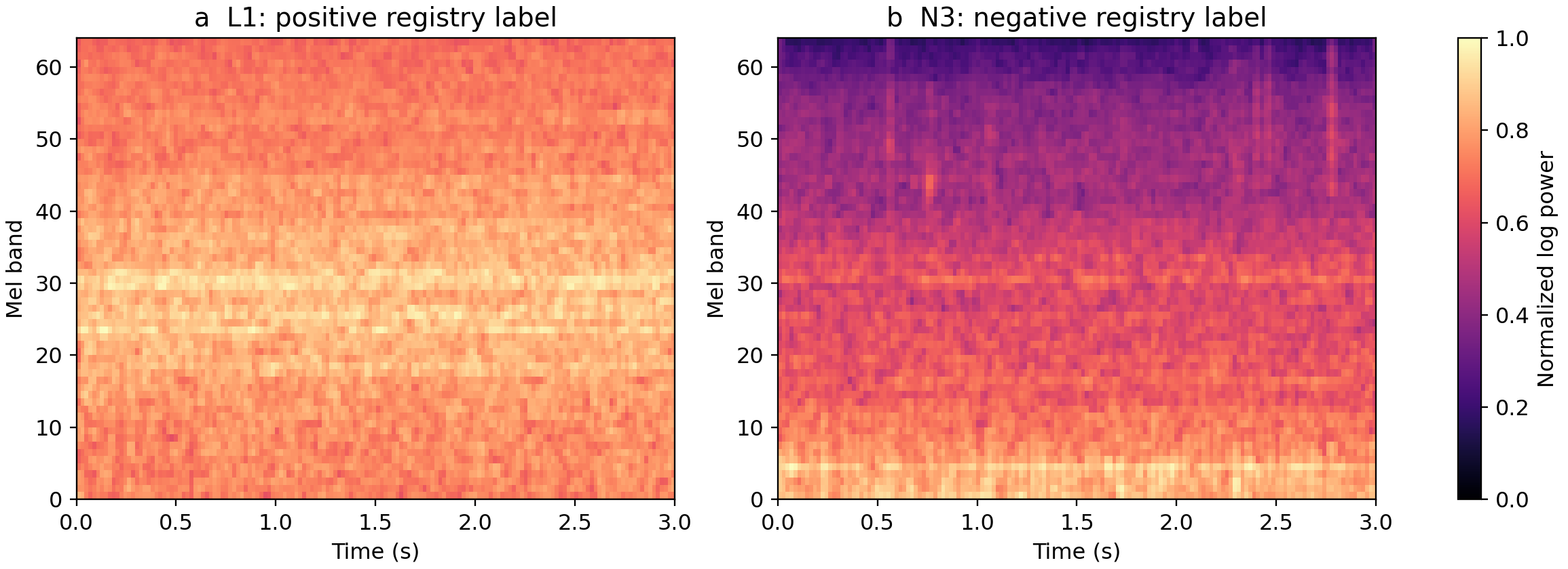
Fig. 1. Examples of the actual network input for registry-positive subset L1 (a) and registry-negative subset N3 (b). The middle resolution is shown after the shared bandpass filter and extraction of a 3 s segment: 6554 Hz, FFT length 512, hop size 128, and 64 Mel bands. Color represents log power relative to each spectrogram's maximum, mapped to [0, 1].
Normalization to each spectrogram's maximum removes a global amplitude scaling factor, including a linear gain change, but discards information about absolute digital RMS. In this SebaKMT corpus, positive subsets () have mean RMS levels between −15.9 and −1.4 dBFS, whereas negative subsets (–) have lower mean levels, between −35.0 and −27.6 dBFS. After normalization, a quiet narrowband background reaches the same maximum color value as an intense positive recording (Figure 1b).
2.3. Neural Architectures and Conventional Baselines
Three architectures are compared to distinguish the effect of multiple spectral resolutions from that of increased parameter count (Figure 2):
- Single-scale CNN, 25,633 parameters. The input is the middle-resolution spectrogram (). One convolutional branch contains 23,520 parameters and three blocks with 16, 32, and 64 channels. Each block uses a convolution, batch normalization, ReLU activation, and pooling. Global average pooling produces a 64-element feature vector. A two-layer classifier comprises , ReLU, dropout with , and . The classifier contains 2,113 parameters, giving 25,633 overall.
- Three-resolution TFCNN, 76,769 parameters. Three independent branches, each containing 23,520 parameters, process resolutions . Their three 64-element vectors are concatenated into a 192-element representation. The classifier comprises , ReLU, dropout with , and , totaling 6,209 parameters. The network therefore contains parameters.
- Capacity control, 76,769 parameters. The three-branch topology and parameter count match TFCNN, but all branches receive the same middle-resolution input, .
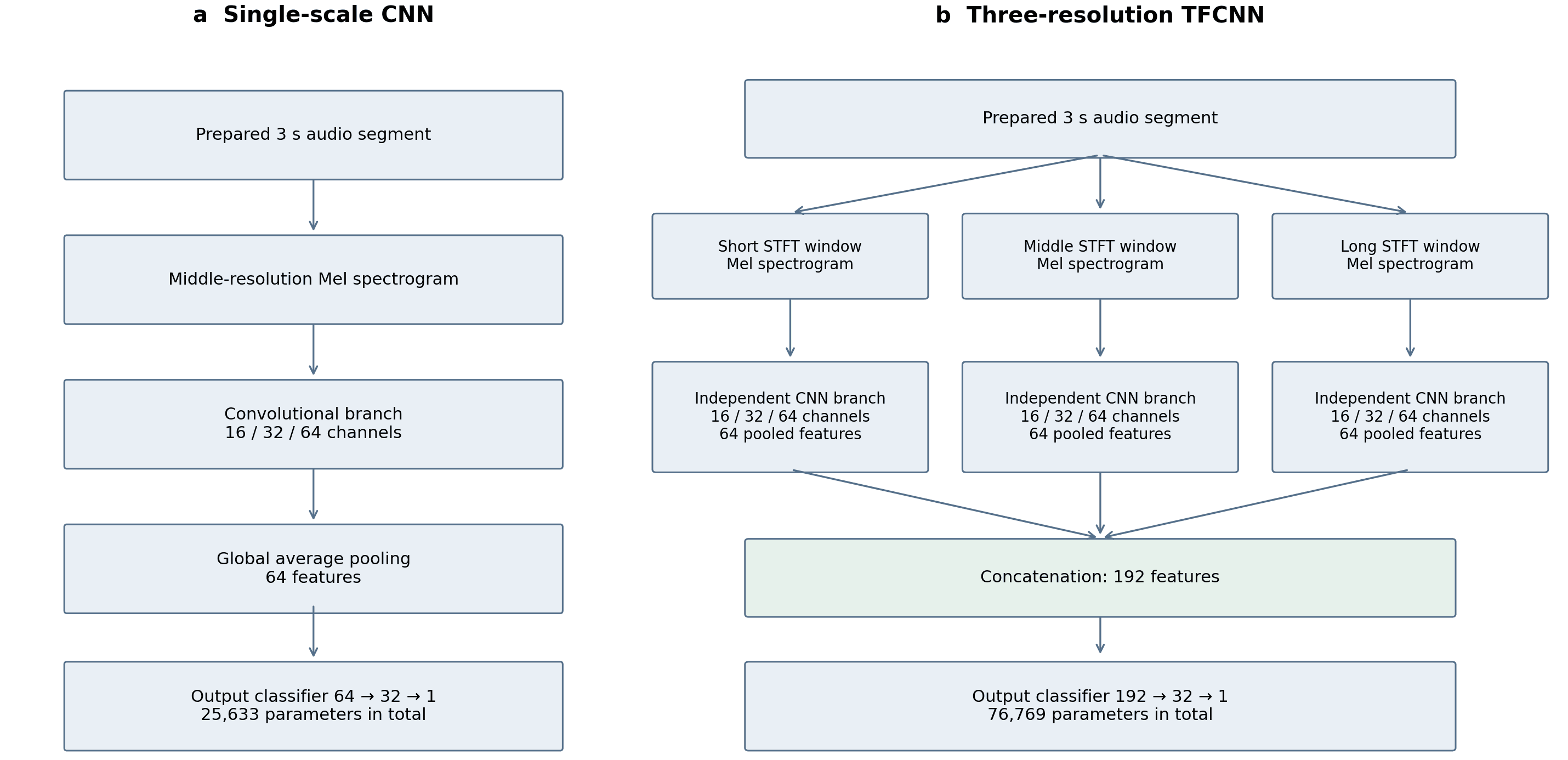
Fig. 2. Single-scale CNN (a, 25,633 parameters) and three-resolution TFCNN (b, 76,769 parameters). The capacity control uses the topology in panel b but supplies the middle-resolution spectrogram to every branch. A file score is the arithmetic mean of sigmoid outputs across its 3 s windows.
Two conventional baselines were also evaluated on the primary SebaKMT corpus: logistic regression with regularization and standardized features, and a random forest with 100 trees. Ten signal features were computed per WAV file: , crest factor, zero-crossing rate, Wiener spectral flatness over 50–3000 Hz, spectral centroid, spectral bandwidth, and four relative energy fractions over 50–150, 150–400, 400–1000, and 1000–3000 Hz. Spectral features were derived using Welch's method with 1,024-sample windows.
The baselines used three feature configurations to examine the potential role of digital level as a shortcut:
- Amplitude only, comprising .
- Nine shape descriptors excluding . This is a separate control without an explicit digital-level feature; it is not equivalent to changing CNN normalization.
- All ten features, including .
3. Data and Evaluation Protocols
3.1. Audit of the Source Collection
The source collection from other instruments initially contained several problems common to unstructured operational archives:
- Of 203 training and validation WAV files, only 141 were byte-unique. File and decoded-sample SHA-256 checks identified 62 exact duplicates stored under different names or paths.
- Before deduplication, 31 of 61 validation files had identical copies in training. They accounted for approximately 54% of validation duration, or 3,441 of 6,345 s.
- Conflicting labels, dependence between sample rate and class, and approximately 100 procedurally generated records with nonphysical spectral templates were also identified in the negative folder.
After deduplication, exclusion of generated records, quarantine of disputed labels, and stratified partitioning, the curated collection contained 136 unique recordings. Standard-profile quality control retained 133 files, yielding 6,380 three-second windows: 88 training files (3,907 windows), 24 validation files (1,419 windows), and 21 test files (1,054 windows; 14 positive and seven negative files).
3.2. SebaKMT Field Recordings and Group Structure
The target collection comprises SebaKMT Correlux / K-2 field recordings attributed through correlator project files and an operational registry. Standard-profile files are sampled at 6554 Hz and last approximately 3.12 s. Each provides one complete 3 s window; the remaining approximately 0.125 s is unused. Low-frequency files are sampled at 1638 Hz and last 12.50 s, providing seven overlapping 3 s windows per file.
The primary target corpus contains 180 standard-profile recordings from six site groups, with 60 positive and 120 negative registry labels. Additional analyses consider 30 low-frequency recordings of one leak event and 39 auxiliary recordings with historical labels.
In the primary corpus, subsets and were recorded on supply pipes within the same large network junction and were assigned to one site group. The auxiliary collection contains subsets and , totaling 39 WAV files.
Short recordings from one session share acquisition conditions. The primary corpus contains seven registry subsets across six site groups and three registered leak events. The WAV count is not the number of independent field trials. Separation was established using registered identifiers, without an independent geospatial survey of all physical connections.
3.3. Experimental and Statistical Protocols
Three sequential protocols were used:
- Protocol A, direct transfer between collections. The single-scale CNN, capacity control, and TFCNN were developed on the curated source corpus of 133 files with ten random initializations, seeds 42–51. Thresholds were fixed using source validation data. Without target fine-tuning, the models were evaluated on 150 SebaKMT files: 50 positive recordings, comprising 20 from and 30 from , and 100 negative recordings from . The retained analysis compared architectures using paired two-sided Student's -tests across seeds with Holm–Bonferroni correction.
- Protocol B, threshold selection and classifier adaptation. Original pretrained weights and an adapted output classifier were compared on fixed SebaKMT partitions.
- In the standard profile, training comprised 79 accepted files: (20), (20), (20), and (19). Validation comprised (20) and (40). Testing comprised (20), (20), and (40). The classifier was fine-tuned for 15 epochs while convolutional branches were frozen. The historical positive label of was not independently verified, so test metrics describe agreement with registry labels. The threshold was selected subject to .
- The low-frequency profile used 30 training, 50 validation, and 50 test files. The 30 recordings of event were partitioned by sensor: ten from sensor 1 for training, ten from sensor 2 for validation, and ten from sensor 3 for testing. All three sensors recorded the same event on the same main. Relative to generalization to a new leak event, this design therefore contains within-event data leakage.
- Protocol C, training from scratch on SebaKMT data with random-file and site-group partitions. All TFCNN parameters and the conventional baselines were trained using the 180-file primary corpus. Both partitioning strategies used 60 training, 60 validation, and 60 test files, with 20 positive and 40 negative files per partition.
- Site-disjoint evaluation used three rotating blocks and ten seeds, giving 30 TFCNN models. Block A contained (20), (20), and (20), keeping the two subsets from the large junction together. Block B contained (20) and (40). Block C contained (20) and (40). Each block served in turn as training, validation, and testing. For each seed, predictions from the three external test blocks were combined into an out-of-fold assessment of all 180 files.
- A random-file control used the same corpus and class counts with a 60/60/60 partition and ten seeds. Training settings were matched: AdamW, dropout 0.2 rather than the original architecture's 0.3, at most 60 epochs, early stopping after ten epochs without improvement in class-balanced file-level validation cross-entropy, and a threshold satisfying .
The standard deviation across ten seeds characterizes optimization variability at fixed partitions. Accuracy across the seven registry subsets is reported descriptively. Two subsets share a site, and some subsets combine multiple recorded series; they are not seven independent field trials. No confidence interval for performance at future sites is inferred from these subset summaries.
4. Results
4.1. Direct Transfer Between Collections Under Protocol A
Table 1 and Figure 3 summarize direct transfer to 150 SebaKMT files: 50 positive recordings, comprising 20 from and 30 from low-frequency main , and 100 negative recordings from . An always-negative classifier provides a reference accuracy of 66.67% because of the 1:2 class ratio, with balanced accuracy (BA) of 50.00%.
Table 1. Direct transfer from the source collection to 150 SebaKMT WAV files without target adaptation. Values are mean ± SD across ten seeds, 42–51, unless only a mean is shown.
| Architecture | Parameters | Accuracy, % | Sensitivity, % | Specificity, % | False positives / 100 negatives | Balanced accuracy, % | Low-frequency true positives / 30 |
|---|---|---|---|---|---|---|---|
| Single-scale CNN | 25,633 | 49.33 ± 26.24 | 78.20 ± 7.21 | 34.90 ± 38.90 | 65.1 ± 38.9 | 56.55 | 19.1 ± 3.6 (63.7%) |
| Capacity control (one scale repeated three times) | 76,769 | 35.60 ± 20.09 | 73.80 ± 6.43 | 16.50 ± 32.70 | 83.5 ± 32.7 | 45.15 | 18.0 ± 5.0 (60.0%) |
| Multiscale TFCNN | 76,769 | 39.80 ± 18.86 | 86.40 ± 8.21 | 16.50 ± 28.10 | 83.5 ± 28.1 | 51.45 | 23.2 ± 4.1 (77.3%) |
| Always-negative reference | 0 | 66.67 | 0.00 | 100.00 | 0.0 | 50.00 | 0.0 (0.0%) |
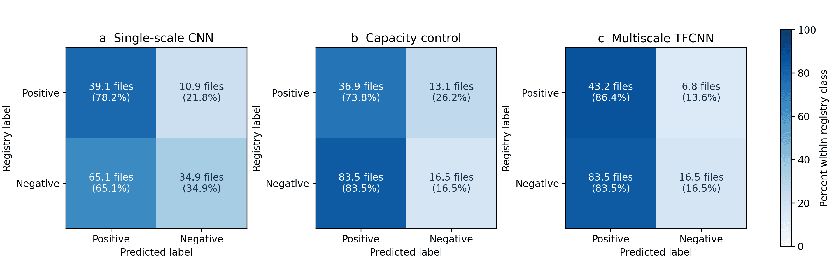
Fig. 3. Mean confusion matrices across ten seeds for direct transfer to 150 SebaKMT files with 50 positive and 100 negative labels. Panels show the single-scale CNN (a, 25,633 parameters), repeated-scale capacity control (b, 76,769 parameters), and multiscale TFCNN (c, 76,769 parameters).
The retained results support two observations:
- Sensitivity with multiple spectral resolutions. Mean sensitivity across all 50 positive recordings increased from 78.20 ± 7.21% for the single-scale model to 86.40 ± 8.21% for TFCNN. The retained paired test gave , , which does not meet the 5% significance criterion. Sensitivity was also higher than for the equal-size capacity control, 73.80 ± 6.43%, with unadjusted , . On the 1,000 mm low-frequency main , TFCNN detected a mean of 23.2 ± 4.1 of 30 positive files (77.3%), compared with 19.1 ± 3.6 (63.7%) for the single-scale model (, ) and 18.0 ± 5.0 (60.0%) for the capacity control (, ). TFCNN used three resolutions, including a 312.6 ms window with 3.2 Hz frequency-bin spacing. For a family of six paired comparisons, however, Holm–Bonferroni correction raises the smallest unadjusted to . This exceeds , so the observation is exploratory.
- Low specificity and substantial seed variation. The single-scale CNN produced 65.1 ± 38.9 false positives per 100 negative files, compared with 83.5 ± 28.1 for TFCNN. Specificity was 34.90% and 16.50%, respectively; the retained comparison was not statistically significant (, ). Balanced accuracy was 56.55% for the single-scale model and 51.45% for TFCNN. At these operating points, direct transfer did not provide performance suitable for practical deployment.
4.2. Threshold Selection and Supervised Adaptation Under Protocol B
Table 2 compares the pretrained TFCNN, threshold adjustment, and output-classifier adaptation on fixed target partitions. The standard-profile test contains 40 positive-labeled files from and and 40 negative-labeled files from . The low-frequency test contains ten files from a held-out sensor recording event and 40 resampled negative files from . Validation and test ROC-AUC are reported alongside threshold-dependent outcomes.
Table 2. Pretrained TFCNN, target-validation threshold selection, and supervised classifier adaptation on SebaKMT recordings. Adapted results summarize ten seeds, except for the explicitly post hoc seed-42 illustration.
| Profile (sample rate) | Model configuration | Threshold | Test TP | Test FP | Sensitivity, % | Specificity, % | BA, % | Validation ROC-AUC, % | Test ROC-AUC, % |
|---|---|---|---|---|---|---|---|---|---|
| Standard (6554 Hz) | Pretrained, stored threshold | 0.6905 | 40 / 40 | 19 / 40 | 100.0 | 52.50 | 76.25 | 81.00 | 92.50 |
| Standard (6554 Hz) | Pretrained, validation-selected threshold | 0.3025 | 40 / 40 | 20 / 40 | 100.0 | 50.00 | 75.00 | 81.00 | 92.50 |
| Standard (6554 Hz) | Adapted classifier (ten seeds), rule | 0.0667 ± 0.0015 | 40 / 40 | 20 / 40 | 100.0 | 50.00 | 75.00 | 78.36 ± 0.21 | 94.16 ± 0.03 |
| Standard (6554 Hz) | Adapted classifier (seed 42), post hoc test threshold 0.78 | 0.7800 | 37 / 40 | 3 / 40 | 92.50 | 92.50 | 92.50 | 78.38 | 94.19 |
| Low frequency (1638 Hz) | Pretrained, stored threshold | 0.5562 | 10 / 10 | 14 / 40 | 100.0 | 65.00 | 82.50 | 93.00 | 98.50 |
| Low frequency (1638 Hz) | Pretrained, validation-selected threshold | 0.5031 | 10 / 10 | 17 / 40 | 100.0 | 57.50 | 78.75 | 93.00 | 98.50 |
| Low frequency (1638 Hz) | Adapted classifier (ten seeds), rule | 0.3817 ± 0.0050 | 10 / 10 | 15 / 40 | 100.0 | 62.50 | 81.25 | 99.97 ± 0.08 | 98.75 ± 0.00 |
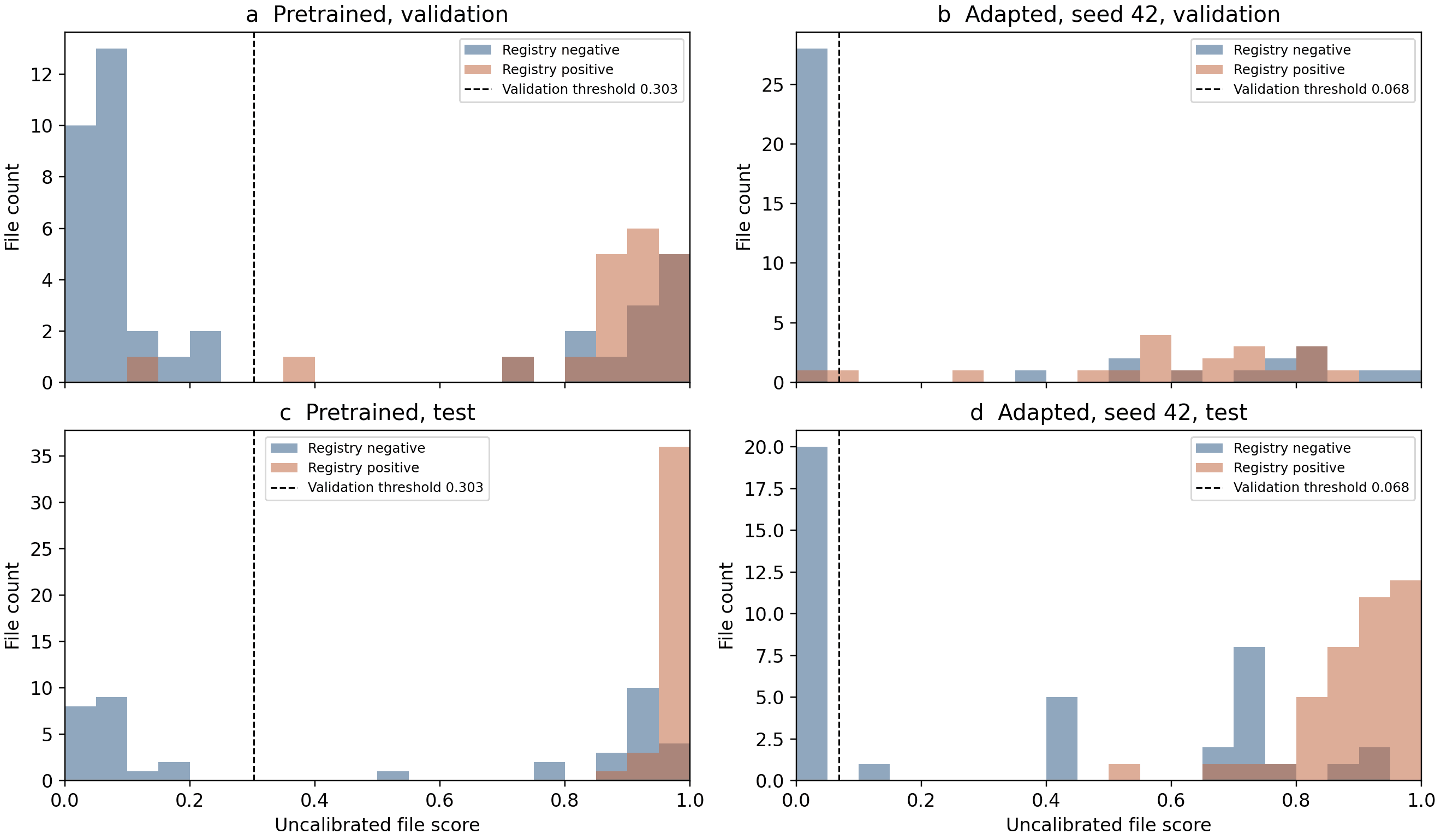
Fig. 4. File-score distributions in the standard profile before and after output-classifier adaptation. The upper row shows validation (60 WAV files); the lower row shows testing (40 positive-labeled and 40 negative-labeled files). Columns show the pretrained model and the adapted model for seed 42. Blue and orange indicate negative and positive registry labels. Dashed lines mark thresholds selected on validation subject to sensitivity of at least 95%.
Two aspects of performance should be distinguished:
- Test-score ranking. Before adaptation, 20 files from one of the two recorded series in negative subset had scores between 0.50 and 1.00, overlapping the positive class; test ROC-AUC was 92.50%. After classifier adaptation, test ROC-AUC increased to 94.16 ± 0.03%. In seed 42, most of these background scores shifted to approximately 0.40–0.76. Three negative files remained above 0.78, with scores of 0.897, 0.912, and 0.937, while 37 of 40 positive-labeled files lay between 0.79 and 0.99. A threshold of 0.78 would produce 37/40 true positives and 3/40 false positives, corresponding to 92.50% sensitivity, specificity, and balanced accuracy. This threshold was examined after inspecting the test data and is not an independently validated operating rule.
- Sensitivity of threshold selection to low-scoring validation records. Every adapted run produced 20 false positives among 40 negative test files at its validation-selected threshold. Two positive-labeled validation files from (
zelenaya,040007AC01.wavand040007AC04.wav) received scores of 0.0242 and 0.0935 in seed 42. They do not belong to disputed subset , and a low score alone does not demonstrate a labeling error. With 20 positive validation files, the requirement permits only one missed file. The selected threshold must therefore include at least the second-lowest positive score. Across seeds, the threshold was . All 20 files from the higher-scoring negative series in , with test scores between 0.126 and 0.937, exceeded this threshold.
4.3. Training from Scratch and Comparison with Conventional Baselines Under Protocol C
To assess performance without the source collection, all TFCNN parameters were trained from scratch using SebaKMT recordings. Preliminary random-file experiments had produced test accuracies of 99.5–100%.
The curated 180-file corpus, containing 60 positive and 120 negative labels, was then used to compare random-file partitioning with three-block site-disjoint evaluation. Ten seeds per grouped split produced 30 TFCNN models. Conventional baselines used the same grouped splits and three feature configurations: digital RMS alone, nine handcrafted signal descriptors without RMS, and all ten features. Table 3 and Figure 5 summarize the comparison.
Table 3. TFCNN and conventional baselines on the 180-file SebaKMT corpus. TFCNN includes random-file and site-group protocols; conventional baselines use the grouped splits. Seed-dependent results summarize seeds 42–51.
| Model and partitioning protocol | Features | Decision rule | Sensitivity, % | Specificity, % | Accuracy, % | BA, % | Within-fold ROC-AUC, % | Pooled ROC-AUC, % |
|---|---|---|---|---|---|---|---|---|
| TFCNN (random-file control) | Three-resolution Mel | 100.0 ± 0.0 | 100.0 ± 0.0 | 100.0 ± 0.0 | 100.0 ± 0.0 | 100.0 ± 0.0 | 100.0 ± 0.0 | |
| TFCNN (site groups) | Three-resolution Mel | 92.67 ± 5.10 | 85.42 ± 5.22 | 87.83 ± 3.22 | 89.04 ± 2.85 | 94.28 ± 3.87 | 90.18 ± 2.60 | |
| TFCNN (site groups) | Three-resolution Mel | Fixed 0.50 | 91.83 ± 5.52 | 63.25 ± 13.72 | 72.78 ± 9.15 | 77.54 ± 7.14 | 94.28 ± 3.87 | 90.18 ± 2.60 |
| Logistic regression | only (1) | Fixed 0.50 | 83.33 | 100.00 | 94.44 | 91.67 | 99.67 ± 0.58 | 95.44 |
| Logistic regression | only (1) | 83.33 | 91.67 | 88.89 | 87.50 | 99.67 ± 0.58 | 95.44 | |
| Random forest | only (1) | Fixed 0.50 | 83.33 ± 0.00 | 100.00 ± 0.00 | 94.44 ± 0.00 | 91.67 ± 0.00 | 91.67 ± 0.00 | 91.53 ± 0.06 |
| Random forest | only (1) | 95.00 ± 3.51 | 33.33 ± 0.00 | 53.89 ± 1.17 | 64.17 ± 1.76 | 91.67 ± 0.00 | 91.53 ± 0.06 | |
| Logistic regression | Handcrafted descriptors (9) | Fixed 0.50 | 98.33 | 82.50 | 87.78 | 90.42 | 97.04 ± 5.12 | 97.85 |
| Logistic regression | Handcrafted descriptors (9) | 98.33 | 82.50 | 87.78 | 90.42 | 97.04 ± 5.12 | 97.85 | |
| Random forest | Handcrafted descriptors (9) | Fixed 0.50 | 53.50 ± 5.64 | 92.25 ± 0.40 | 79.33 ± 1.61 | 72.88 ± 2.62 | 95.74 ± 0.18 | 94.41 ± 0.85 |
| Random forest | Handcrafted descriptors (9) | 85.83 ± 4.86 | 91.25 ± 1.13 | 89.44 ± 1.92 | 88.54 ± 2.61 | 95.74 ± 0.18 | 94.41 ± 0.85 | |
| Logistic regression | All features (10) | Fixed 0.50 | 100.00 | 90.00 | 93.33 | 95.00 | 99.42 ± 1.01 | 99.81 |
| Logistic regression | All features (10) | 100.00 | 91.67 | 94.44 | 95.83 | 99.42 ± 1.01 | 99.81 | |
| Random forest | All features (10) | Fixed 0.50 | 84.50 ± 3.69 | 93.00 ± 1.31 | 90.17 ± 1.41 | 88.75 ± 1.87 | 96.13 ± 0.00 | 98.03 ± 0.86 |
| Random forest | All features (10) | 84.50 ± 3.69 | 94.17 ± 3.69 | 90.94 ± 2.16 | 89.33 ± 1.89 | 96.13 ± 0.00 | 98.03 ± 0.86 |
For CNN and random forest, ± denotes sample SD across ten seeds. For within-fold ROC-AUC of deterministic logistic regression, ± denotes SD across the three folds. These quantities describe different sources of variation and are not directly comparable. Pooled ROC-AUC combines scores from separately trained models and is provided descriptively.
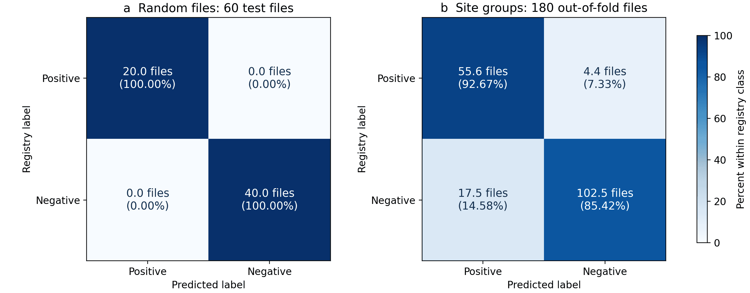
Fig. 5. Mean confusion matrices across ten seeds for TFCNN trained from scratch on SebaKMT recordings. Random-file partitioning uses 60 test files (a); site-group partitioning combines external predictions for 180 files (b). Percentages are normalized within each registry class.
Five observations follow:
- Evaluation protocol. The random-file control achieved 100% accuracy. Grouped evaluation yielded accuracy of 87.83 ± 3.22%, sensitivity of 92.67 ± 5.10%, and specificity of 85.42 ± 5.22%. Mean errors were 17.50 ± 6.26 false positives among 120 negative files and 4.40 ± 3.06 false negatives among 60 positive files. The 12.17 percentage-point accuracy difference describes these protocols with different test compositions; it does not isolate a causal effect of session overlap. Conventional models were evaluated only on the grouped splits in this analysis.
- Baseline model comparison. Logistic regression using nine handcrafted signal descriptors achieved an accuracy similar to that of TFCNN (87.78% vs. 87.83 ± 3.22%), with higher sensitivity (98.33% vs. 92.67%) but lower specificity (82.50% vs. 85.42%). These results do not establish an accuracy advantage for the deep architecture on this corpus. Logistic regression on digital RMS alone reached 94.44% accuracy at threshold 0.50 (within-fold ROC-AUC 99.67 ± 0.58%), though with lower sensitivity (83.33% vs. 92.67%). Digital RMS was strongly predictive of registry labels, motivating further investigation of acquisition-related shortcuts rather than demonstrating a physical acoustic mechanism.
- Descriptive variation across subsets. Unweighted mean accuracy across the seven registry subsets was 87.07%, with an SD of 17.21 percentage points between subset means. This describes heterogeneity in the current corpus and is not a confidence interval for future sites.
- Digital level and possible amplitude limiting. In , a mean of 51.89% of samples had an absolute amplitude of at least 0.99 full scale, and the mean crest factor was 1.18. Only 1.99% of samples had an absolute raw code of exactly 32688. These are distinct quantities. The waveform is consistent with amplitude limiting, but its origin in the analog-to-digital converter, analog signal chain, digital processing, or export cannot be established. The quality-control threshold of 0.999 does not detect these near-full-scale samples. Predictive digital RMS may reflect signal intensity, acquisition conditions, or both; gain settings were not recovered from the WAV files.
- Threshold selection for TFCNN. With a fixed threshold of 0.50, predictions from the three grouped models yielded 63.25% specificity and 72.78% accuracy. Selecting a threshold on each validation block subject to sensitivity of at least 95% adjusted the operating point and yielded 87.83% overall accuracy.
Table 4. Acoustic characteristics and out-of-fold accuracy across seven registry subsets.
| Subset | WAV | Registry label | RMS, dBFS | Crest factor | Maximum absolute amplitude | Samples ≥ 0.99 full scale, % | TFCNN accuracy, % [min; max] | Logistic regression accuracy, % |
|---|---|---|---|---|---|---|---|---|
| 20 | Positive | -1.45 ± 0.26 | 1.18 ± 0.04 | 0.9976 | 51.89 ± 8.43 | 98.5 [85.0; 100.0] | 100.0 | |
| 20 | Positive | -15.87 ± 9.91 | 2.60 ± 0.89 | 0.9976 | 1.78 ± 1.85 | 96.5 [65.0; 100.0] | 100.0 | |
| 20 | Positive | -9.83 ± 5.43 | 2.76 ± 1.48 | 0.9980 | 5.26 ± 5.46 | 83.0 [50.0; 90.0] | 100.0 | |
| 20 | Negative | -27.56 ± 1.59 | 3.28 ± 0.65 | 0.2004 | 0.00 ± 0.00 | 100.0 [100.0; 100.0] | 100.0 | |
| 40 | Negative | -31.09 ± 4.47 | 3.69 ± 0.81 | 0.2493 | 0.00 ± 0.00 | 93.0 [47.5; 100.0] | 100.0 | |
| 40 | Negative | -34.95 ± 3.78 | 4.27 ± 0.86 | 0.1247 | 0.00 ± 0.00 | 88.0 [80.0; 97.5] | 75.0 | |
| 20 | Negative | -31.78 ± 0.80 | 3.87 ± 0.90 | 0.1242 | 0.00 ± 0.00 | 50.5 [50.0; 55.0] | 100.0 |
Logistic regression uses all ten features and thresholds selected only on validation. Correct predictions summed across subsets are 170/180 (94.44%), with ten false positives and no false negatives, matching Table 3. At a fixed threshold of 0.50, accuracy on is 90% and the total is 168/180 (93.33%). SDs of RMS, crest factor, and the high-amplitude sample fraction are calculated across files. The high-amplitude sample mean is expressed as a percentage and its SD in percentage points.
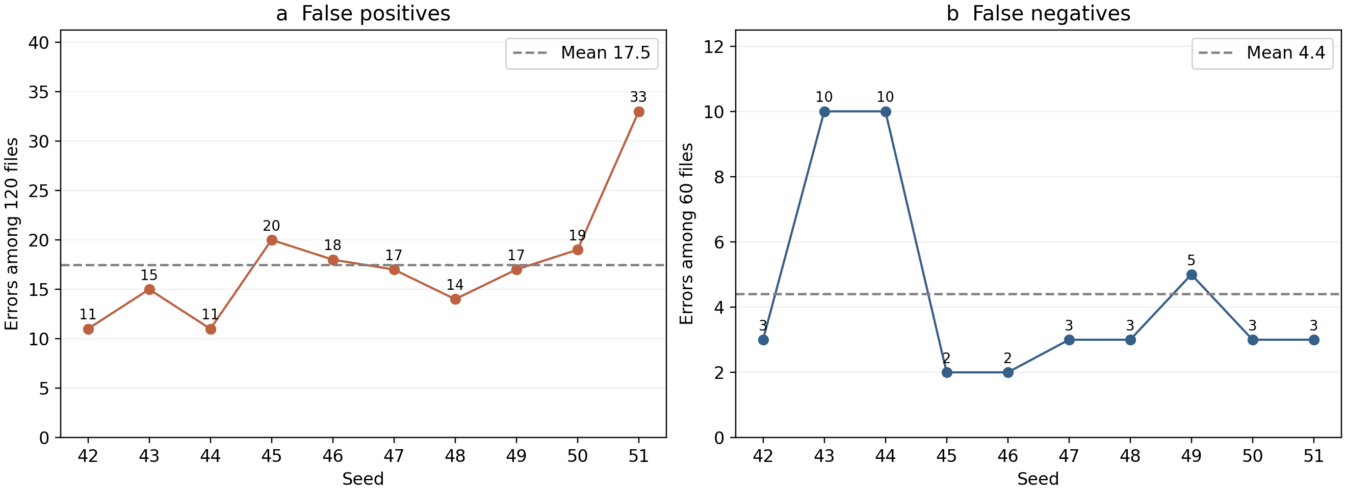
Fig. 6. Out-of-fold errors across ten random initializations, seeds 42–51, under grouped evaluation of 180 WAV files. Panels show false positives among 120 negative files (a, mean 17.5) and false negatives among 60 positive files (b, mean 4.4).
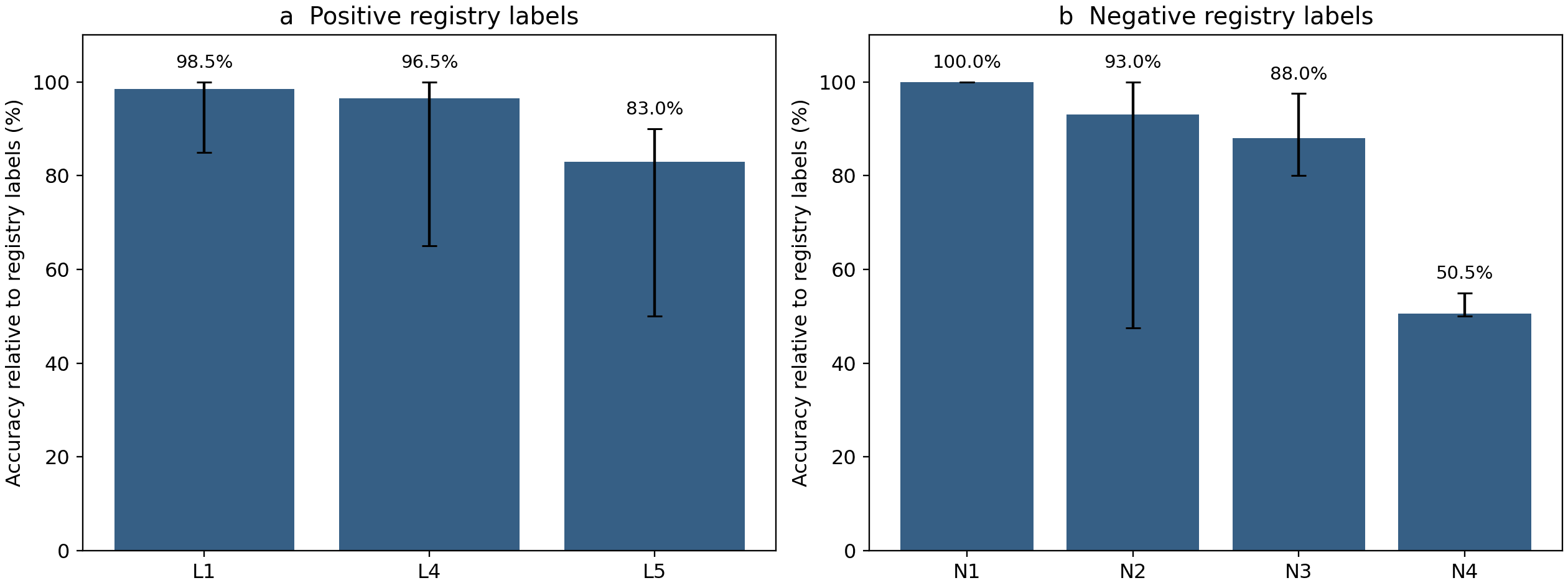
Fig. 7. TFCNN accuracy across seven registry subsets under grouped evaluation. Bars indicate means across ten seeds; whiskers span the minimum and maximum. Panels show subsets with positive (a) and negative (b) registry labels. These subsets are not seven independent sites.
The subset analysis identifies three additional patterns:
- Fewer alarms on after training from scratch. Under classifier adaptation in Protocol B, produced 20 alarms among 40 negative-labeled files (50.0%). In grouped split 3, with excluded from both training and validation, training from scratch produced 4.80 ± 3.08 false positives among these 40 files (12.00%), with fold ROC-AUC of 94.67 ± 1.75%.
- Heterogeneity within . TFCNN produced 9.90 ± 0.32 alarms among 20 files, ranging from nine to ten. Alarms were concentrated on sensor A; sensor B produced none. The source of this asymmetry remains unresolved. The current ten-feature logistic regression produced two alarms on at threshold 0.50 and none at its validation-selected threshold. It therefore did not reproduce the same ten alarms as TFCNN.
- Early-stopping instability with few events. In grouped split 2, seeds 42–50 produced zero to four false positives among 40 negative files in , with test ROC-AUC of 97.9–100.0%. For seed 51, validation on block A selected the first-epoch checkpoint; test ROC-AUC was 65.5%, with 21 false positives among 40 files. This contributes to the peak of 33 overall false positives in Figure 6a. Each training partition contains only one positive event, represented by 20 WAV files, making epoch and threshold selection sensitive to initialization and the single validation event.
4.4. Auxiliary Field Recordings T1 and T2
After models and thresholds had been fixed, an auxiliary analysis was performed on 39 recordings excluded from training these 40 models. The files had been used in earlier development, and their physical grouping and labels were not independently verified. This is therefore neither a new blind evaluation nor an established independent out-of-distribution test.
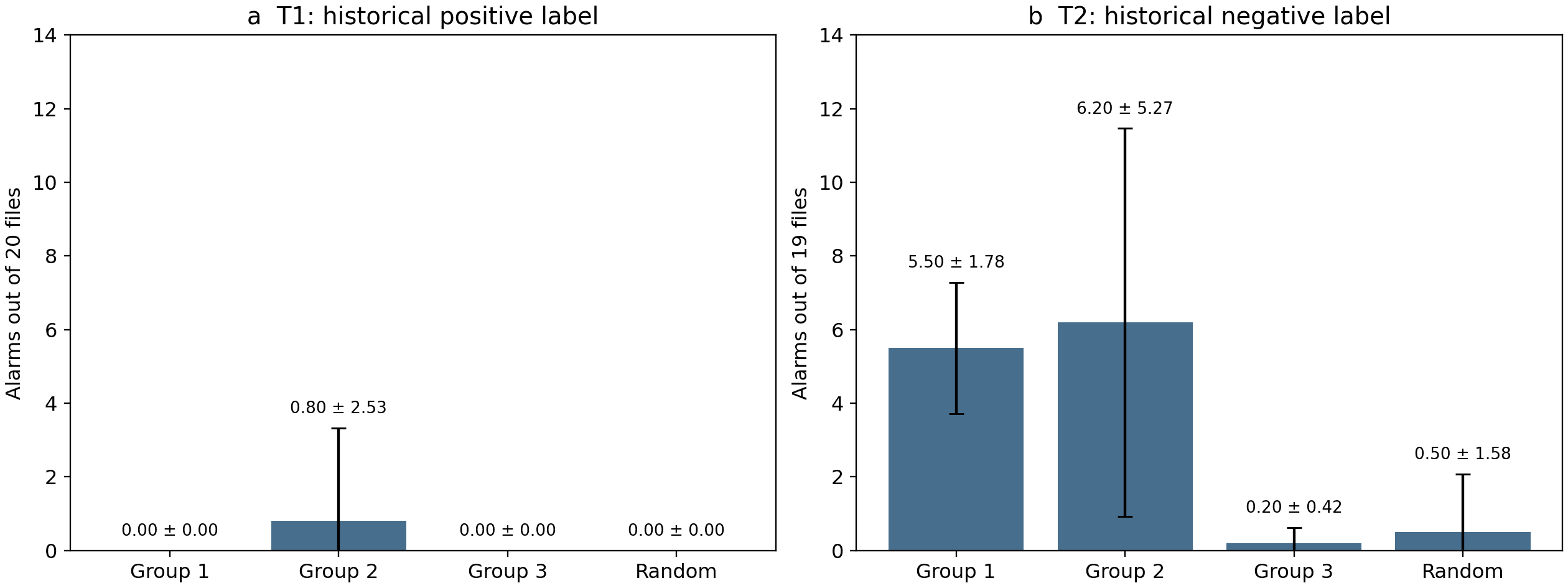
Fig. 8. Alarm counts on auxiliary subsets T1 (a, 20 WAV files) and T2 (b, 19 WAV files). Bars and error bars indicate means and sample SDs across ten seeds for each split. Historical labels are not treated as independently verified ground truth.
- Subset T1. These 20 historically positive-labeled recordings contain a prominent tone near 96 Hz. After the subset was excluded from training, 39 of 40 models produced no alarms and one produced eight. This change relative to earlier runs establishes neither the physical source of the signal nor memorization of that particular tone. Without label verification, it cannot be interpreted as a confirmed leak miss rate.
- Subset T2. For the 19 historically negative-labeled recordings, mean alarm counts were 5.50 ± 1.78, 6.20 ± 5.27, and 0.20 ± 0.42 for the three grouped splits, and 0.50 ± 1.58 for the random control. These are alarm counts relative to historical labels, not independently verified false-alarm rates.
5. Discussion
5.1. Distribution Shift and Digital Signal Level
Direct transfer changes the instrument, pipe section, background, and acquisition conditions together. Peak normalization removes a global digital amplitude factor but does not make different measurement systems equivalent. Its contribution to network errors remains a hypothesis because a paired normalization ablation was not performed in this comparison.
Conventional models show that digital RMS is associated with registry class in this corpus. Its predictive performance does not establish a universal physical relationship or identify the cause of the level difference. Digital dBFS is not calibrated sound pressure. Peak normalization also preserves waveform distortions introduced by amplitude limiting, which may remain potential shortcut features for a CNN.
Published neural and ensemble approaches [4–8] use different datasets and acquisition conditions. Their numerical results cannot be directly ranked against this study without examining site composition, evaluation protocols, and label verification. Research on domain shift [12, 13] and normalization [17, 18] provides directions for further investigation but does not establish the cause of the errors observed here.
5.2. Score Ranking and Operating Thresholds
ROC-AUC measures the ranking of model scores relative to labels. In the standard profile, adaptation improved test ROC-AUC to 94.16% but did not reduce alarms on negative-labeled recordings at the validation-selected threshold. Two low scores in validation subset affected the threshold when at least 19 of 20 positive validation files had to be detected. Their low scores do not demonstrate label errors.
A post hoc threshold of 0.78 reduces errors on this test, but it was not selected independently of test labels. Alternative rules, including maximizing Youden's , can be compared using validation data; they do not guarantee stability at a new site. Selecting a threshold is distinct from calibrating model output as a probability. The low-frequency result concerns a sensor recording the same event and does not establish transfer to a new leak.
5.3. Validation Design and Causal Interpretation
Work on grouped validation and data leakage [9–11, 14–16] supports matching data partitioning to the intended application. Random-file partitioning retains familiar acquisition conditions in training and testing. In our comparison, its performance exceeded that obtained when registered site groups were excluded.
This is consistent with the use of session-related features but does not identify the features learned by the network. The random control uses 60 test files, whereas the pooled grouped assessment uses 180; the 12.17 percentage-point difference is not a paired causal estimate. Similarly, comparing classifier adaptation with training from scratch changes both data composition and training settings and does not isolate the benefit or harm of pretraining.
6. Limitations and Future Work
- Event count. The primary corpus contains three registered leak events. Each split places one event in training, one in validation, and one in testing. Epoch and threshold selection depend on one validation event. Seven registry subsets belong to six site groups; seed variation does not quantify uncertainty across future sites.
- Labels and prior exposure. Labels were inherited from the registry and were not independently verified in the field during this study. The adaptation test includes disputed subset . The 39 auxiliary recordings were used in earlier development. Incomplete file-level records of early transfer runs prevent independent reproduction of all paired tests.
- Digital signal level. High digital levels and signs consistent with amplitude limiting motivate investigation of acquisition-related features but do not establish their hardware origin. Gain settings and export parameters are unknown. Waveform changes may survive peak normalization and require controlled investigation.
- Further controls. Future work should prespecify a rule for identifying windows without near-full-scale samples and report the fraction of data retained; assess sensitivity to excluding ; and examine the effects of artificial amplitude limiting on both classes. These controls have not been performed and do not replace new field recordings. Records should not be excluded based on their test predictions.
- Independent evaluation. Performance depends on dataset composition and the selected threshold. Assessing new sites requires independently collected recordings with verified labels and a prespecified protocol. Model weights, processing, thresholds, and metrics should be fixed before inspecting new-site outcomes. Adaptation data must be separated from the final test by event and site. External evaluation should include leaks and diverse background conditions, with quality-control rejections reported separately.
7. Conclusions
- Direct transfer of the three-resolution network increased sensitivity relative to the single-scale model but yielded low specificity and did not establish reliable transfer to new instruments and sites.
- Output-classifier adaptation improved ranking on the standard-profile test but retained 20 alarms among 40 negative-labeled files at the validation-selected threshold. These metrics describe agreement with registry labels, including disputed subset .
- Training from scratch achieved 100% accuracy under random-file partitioning and 87.83 ± 3.22% under grouped evaluation. This contrast demonstrates dependence on evaluation design without establishing a specific memorization mechanism.
- Responses to 39 auxiliary recordings depended on training context. Without verified labels, these results describe alarms rather than confirmed field-diagnostic errors.
- Logistic regression using nine handcrafted signal descriptors achieved an accuracy similar to that of TFCNN (87.78% vs. 87.83 ± 3.22%), with higher sensitivity (98.33% vs. 92.67 ± 5.10%) but lower specificity (82.50% vs. 85.42 ± 5.22%). These results do not establish an accuracy advantage for the deep architecture on this corpus. Logistic regression on digital RMS alone reached 94.44% accuracy at threshold 0.50 and 99.67 ± 0.58% within-fold ROC-AUC, but with lower sensitivity (83.33%), which is a notable operational caveat for leak detection. Digital RMS was strongly predictive of registry labels, motivating further investigation of acquisition-related shortcuts (such as gain settings, converter limits, or export processing) combined with recording anomalies, rather than confirming a physical acoustic mechanism. Site-grouped benchmarks on small datasets should therefore report transparent feature baselines alongside deep models.
Acknowledgments and Declaration of Generative AI Usage
During the preparation of this work, the authors used Generative AI and Large Language Model (LLM) tools solely as an assistive technology for cross-lingual drafting, technical translation from the authors' primary working language, grammatical refinement, and manuscript formatting. All scientific hypotheses, physical and mathematical problem formulations, experimental software implementations, empirical data processing, and analytical conclusions were independently developed, executed, and verified by the authors. The authors retain full personal and academic responsibility for the integrity and content of this publication.
References
- Bykerk, L., Valls Miro, J. (2022). Vibro-Acoustic Distributed Sensing for Large-Scale Data-Driven Leak Detection on Urban Distribution Mains. Sensors, 22(18), 6897. DOI: 10.3390/s22186897.
- Muggleton, J. M., Brennan, M. J., Pinnington, R. J. (2002). Wavenumber prediction of waves in buried pipes for water leak detection. Journal of Sound and Vibration, 249(5), 939–954. DOI: 10.1006/jsvi.2001.3881.
- Muggleton, J. M., Brennan, M. J., Linford, P. W. (2004). Axisymmetric wave propagation in fluid-filled pipes: wavenumber measurements in in vacuo and buried pipes. Journal of Sound and Vibration, 270(1–2), 171–190. DOI: 10.1016/S0022-460X(03)00489-9.
- Gunatilake, A., Valls Miro, J. (2024). Multimodel Neural Network for Live Classification of Water Pipe Leaks From Vibro-Acoustic Signals. IEEE Sensors Journal, 24(9), 14825–14832. DOI: 10.1109/JSEN.2024.3379476.
- Boadu, V., El-Zahab, S., Zayed, T. (2024). Enhancing Automated Acoustic Leak Detection in a Water Distribution Network Using Ensemble Machine Learning. Journal of Water Resources Planning and Management (ASCE), 150(11). DOI: 10.1061/JWRMD5.WRENG-6578.
- Bakhtawar, B., Fares, A., Zayed, T. (2025). AIoT-Driven Leak Detection in Real Water Networks Using Hydrophones. Water Resources Management, 39(6), 2551–2566. DOI: 10.1007/s11269-024-04077-3.
- Kwon, S., Jeon, S., Park, T.-J., Bae, J.-H. (2024). Automatic Weight Redistribution Ensemble Model Based on Transfer Learning to Use in Leak Detection for the Power Industry. Sensors, 24(15), 4999. DOI: 10.3390/s24154999.
- Cheng, J., Jiang, Z., Wu, H., Zhang, X. (2025). Water Pipeline Leak Detection Method Based on Transfer Learning. Water, 17(3), 368. DOI: 10.3390/w17030368.
- Saeb, S., Lonini, L., Jayaraman, A., Mohr, D. C., Kording, K. P. (2017). The need to approximate the use-case in clinical machine learning. GigaScience, 6(5), gix019. DOI: 10.1093/gigascience/gix019.
- Little, M. A., Varoquaux, G., Saeb, S., et al. (2017). Using and understanding cross-validation strategies. Perspectives on Saeb et al. GigaScience, 6(5), gix020. DOI: 10.1093/gigascience/gix020.
- Roberts, D. R., Bahn, V., Ciuti, S., et al. (2017). Cross-validation strategies for data with temporal, spatial, hierarchical, or phylogenetic structure. Ecography, 40(8), 913–929. DOI: 10.1111/ecog.02881.
- Mesaros, A., Heittola, T., Virtanen, T. (2018). A multi-device dataset for urban acoustic scene classification. Proceedings of the Detection and Classification of Acoustic Scenes and Events 2018 Workshop (DCASE2018), 9–13. arXiv:1807.09840.
- Kawaguchi, Y., Imoto, K., Koizumi, Y., et al. (2021). Description and Discussion on DCASE 2021 Challenge Task 2: Unsupervised Anomalous Sound Detection for Machine Condition Monitoring under Domain Shifted Conditions. Proceedings of the DCASE 2021 Workshop, 186–190. arXiv:2106.04492.
- Tougui, I., Jilbab, A., El Mhamdi, J. (2021). Impact of the Choice of Cross-Validation Techniques on the Results of Machine Learning-Based Diagnostic Applications. Healthcare Informatics Research, 27(3), 189–199. DOI: 10.4258/hir.2021.27.3.189.
- Kaufman, S., Rosset, S., Perlich, C., Stitelman, O. (2012). Leakage in data mining: Formulation, detection, and avoidance. ACM Transactions on Knowledge Discovery from Data (TKDD), 6(4), 15. DOI: 10.1145/2382577.2382579.
- Kapoor, S., Narayanan, A. (2023). Leakage and the reproducibility crisis in machine-learning-based science. Patterns, 4(9), 100804. DOI: 10.1016/j.patter.2023.100804.
- Lostanlen, V., Palmer, K., Knight, E., et al. (2019). Per-Channel Energy Normalization: Why and How. IEEE Signal Processing Letters, 26(1), 39–43. DOI: 10.1109/LSP.2018.2878620.
- Li, Y., Wang, N., Shi, J., Hou, X., Liu, J. (2018). Adaptive Batch Normalization for practical domain adaptation. Pattern Recognition, 80, 109–117. DOI: 10.1016/j.patcog.2018.03.005.
- Geirhos, R., Jacobsen, J.-H., Michaelis, C., et al. (2020). Shortcut learning in deep neural networks. Nature Machine Intelligence, 2(11), 665–673. DOI: 10.1038/s42256-020-00257-z.
Citation
This research paper is permanently archived as a preprint on Zenodo:
Ivanaiskii, A., Ivanaiskii, E., & Shipilov, S. (2026). Evaluating Transferability and Validation Protocols of Convolutional Neural Networks for Acoustic Water Leak Detection Using SebaKMT Logger Recordings [Preprint]. Zenodo. https://doi.org/10.5281/zenodo.23446900