Spectral Shortcut Learning and Generalization Degradation in 2D-CNN Spectrogram Classifiers Trained on Physics-Agnostic Procedural Synthetic Data

Abstract

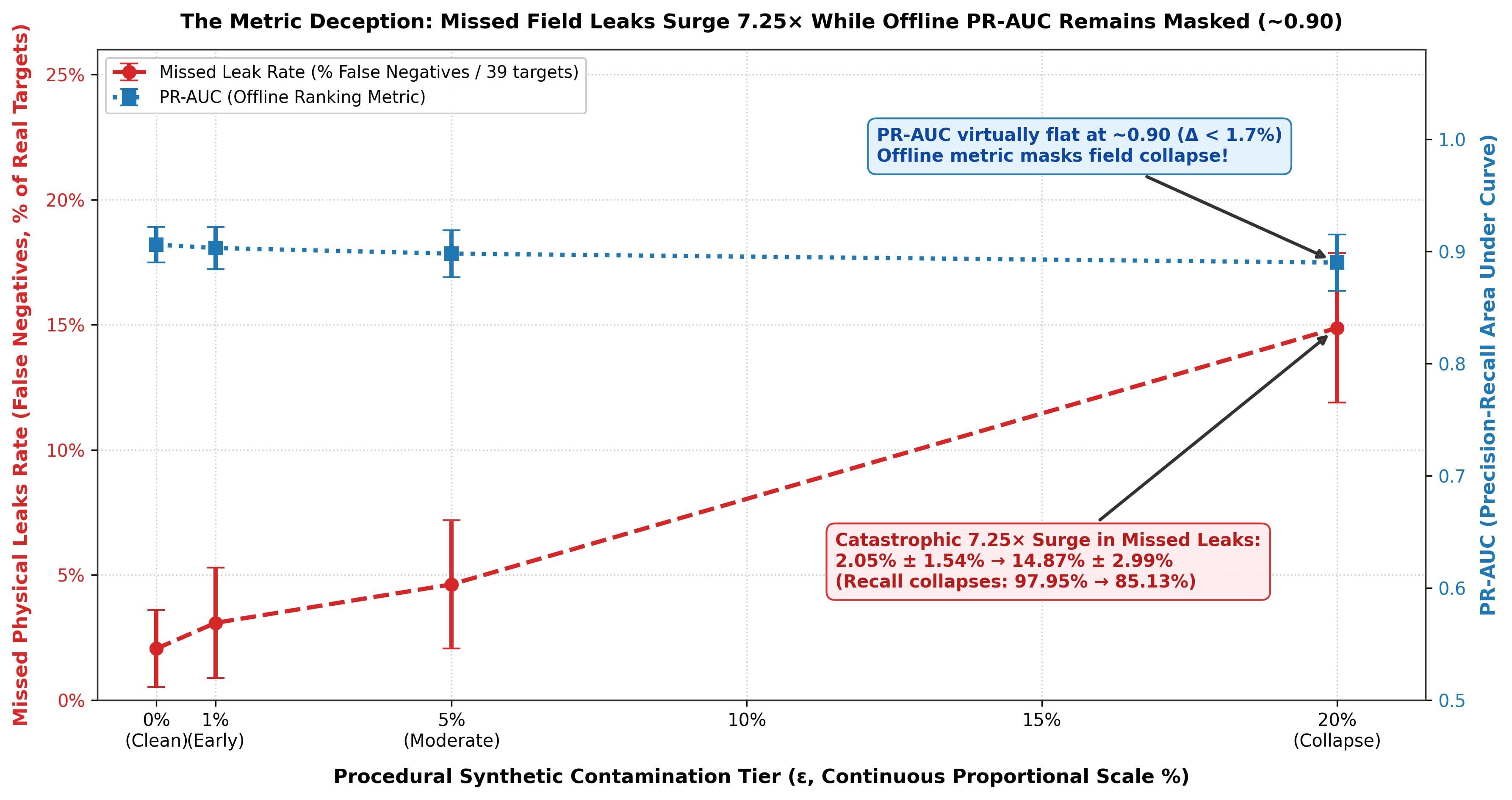
Applying 2D-CNN spectrogram classifiers for acoustic leak detection in fluid-transport pipelines is fundamentally hindered by the acute shortage of field positive leak recordings. An increasingly common practice among NDT practitioners is the rapid generation of surrogate acoustic WAV files using heuristic scripts produced via Large Language Models (LLMs). Such generators (e.g., heuristic parametric waveform generator) synthesize artificial waveforms using simplified correlator equations (additive noise and Gaussian bursts). In this work, employing a rigorous multi-seed statistical benchmark (10 independent random seeds, 40 complete training-evaluation cycles), we systematically examine the generalization dynamics of 2D-CNN spectrogram classifiers under progressive contamination by LLM-assisted procedural synthetic data $\epsilon \in [0.0,0.20]$. Validation is executed on a clean held-out physical validation corpus ($N=61$, 39 leak targets, 22 normal pipes, sampling rate $f_s=44,100\text{ Hz}$). We establish that LLM-assisted procedural surrogate injection triggers Spectral Shortcut Learning and substantial Recall Degradation: at $\epsilon =20\%$, physical leak detection Recall decreases from $97.95\pm 1.54\%$ down to $85.13\pm 2.99\%$, while missed physical leaks surge 7.25-fold (from $0.8\pm 0.6$ to $5.8\pm 1.2$ out of 39 targets under a fixed operating threshold $\tau =0.50$). Convolutional filters selectively adapt to high-contrast narrowband bursts produced by the generator, reducing sensitivity to the stochastic vibroacoustic signatures of genuine field leaks.

Keywords: acoustic emission, pipeline non-destructive testing, spectrogram AI model, Mel-spectrograms, synthetic augmentation, heuristic procedural generators, shortcut learning, recall collapse, statistical benchmark.

---

1. Introduction and Physical Fundamentals

1.1. Physics of Frequency-Dependent Acoustic Wave Attenuation

High-frequency acoustic components ($\ge 5\text{ kHz}$) experience severe attenuation over distances $x>30\text{ m}$, leaving low-amplitude residual spectra ($1-4\text{ kHz}$) at the sensor location, heavily masked by non-stationary hydrodynamic background interferences (pumps, cavitation, regulating valves, transport noise).

The physical origin of accelerated high-frequency attenuation stems from viscoelastic dissipation in the pipe wall and acoustic radiation losses into the surrounding medium (thermal insulation, backfill soil, conduits). According to the Stokes-Kirchhoff dissipation model and elastic wave radiation theory, the attenuation coefficient $\alpha (f)$ scales quadratically with frequency $f$:

$$\alpha (f)=\frac{2{\pi }^2{f}^2}{\rho v^3}\left(\frac{4}{3}\eta +{\eta }_v\right)+{\alpha }_{\text{medium}}(f)$$

where $f$ is the acoustic wave frequency, $\rho$ is the material and fluid density, $v$ is the phase velocity of elastic waves in the pipe wall ($v_{\text{steel}}\approx 5,291\text{ m/s}$), $\eta$ and ${\eta }_v$ denote shear and bulk dynamic viscosities, and ${\alpha }_{\text{medium}}(f)\propto f^{\gamma }$ ($\gamma \ge 1$) represents radiation damping into surrounding media.

Due to the quadratic frequency dependence ($\propto f^2$), acoustic energy above $5\text{ kHz}$ is completely dissipated over tens of meters. Consequently, acoustic NDT sensors capture residual leak emissions strictly within the narrow physical passband of $1-4\text{ kHz}$, where weak defect signatures overlap with operational noise.

1.2. Practical Context and Synthetic Contamination Scenario

In industrial non-destructive testing (NDT) and automated defect detection pipelines, practitioners frequently face the challenge of procedural synthetic audio contamination. To rapidly augment scarce training archives or simulate acceptance test waveforms, heuristic procedural scripts (frequently generated via LLMs) are often employed, synthesizing simplified narrowband bursts in the $2-3\text{ kHz}$ interval designed primarily to satisfy basic cross-correlation benchmarks.

When such surrogate recordings are ingested into centralized data lakes, they risk being unintentionally used to train deep learning models alongside genuine field measurements. While recent studies explore model collapse in LLMs [Shumailov et al., Nature, 2024] and theoretical distribution shift bounds [Dohmatob et al., ICLR, 2025], domain-specific collapse mechanisms in 2D-CNN spectrogram classifiers require quantitative physical investigation.

1.3. Scientific Contributions

In this study, the behavior of 2D-CNN spectrogram classifiers (baseline architecture, 4,217,857 parameters) is evaluated via a 10-seed statistical benchmark (40 full training cycles) on a baseline field acoustic dataset ($N=203$) under varying synthetic contamination $\epsilon \in [0.0,0.20]$, validated on a clean held-out physical split ($N=61$):

1. Clean Baseline Performance ($\epsilon =0\%$): Clean training achieves Recall = $97.95\pm 1.54\%$, Accuracy = $75.74\pm 6.21\%$, and PR-AUC = $0.9061\pm 0.0074$, missing on average only $0.8\pm 0.6$ out of 39 real leaks per evaluation run (8 cumulative misses across 10 seeds).
2. Discovery of Spectral Shortcut Learning and Recall Collapse: At $\epsilon =20\%$, leak detection Recall drops by $12.82\%$ (down to $85.13\pm 2.99\%$), while missed leaks surge 7.25-fold to $5.8\pm 1.2$ defects. Precision exhibits an artifactual increase to $79.18\pm 2.47\%$ due to hyper-conservative decision threshold shifting.
3. Physical-Mathematical Proof of Surrogate Inadequacy: We demonstrate that idealized narrowband bursts produced by procedural scripts disproportionately influence gradient updates, significantly reducing classifier sensitivity to genuine physical leaks.

---

2. Methodology and Experimental Framework

2.1. Spectrogram AI Model Classifier Architecture (Baseline Spectrogram AI Model Classifier)

In acoustic non-destructive testing (NDT), the spectrogram classifier processes two-dimensional logarithmic Mel-spectrograms representing the time-frequency energy distribution of the pipeline vibroacoustic field.

Digital Signal Processing (DSP) Pipeline Parameters:

1. Chunking and Digitization: Continuous acoustic streams are segmented into 3.0-second intervals ($T=3.0\text{ s}$) sampled at $f_s=44,100\text{ Hz}$ ($132,300$ samples per vector).
2. Short-Time Fourier Transform (STFT): A Hann window of length $N_{\text{fft}}=2048$ with a hop length of $H=512$ samples is applied.
3. Log-Mel Filterbank: Power spectra are projected onto $N_{\text{mels}}=128$ triangular Mel filters restricted to the physically active band of $100-4000\text{ Hz}$. This band captures acoustic emissions from pressurized orifice jetting while rejecting high-frequency transducer electrical interference. The input spectrogram matrix dimension is $128\times 256$ (128 frequency bands $\times$ 256 temporal frames).
4. Amplitude Scaling: Power values are converted to decibels ($S_{\text{dB}}=10{\log }_{10}(S/\max (S))$) followed by min-max normalization mapping amplitudes to the continuous interval $[0.0,1.0]$.

Layer-by-Layer Neural Architecture:

The network is partitioned into two distinct functional stages — a convolutional feature extractor (acoustic morphology analysis) and a fully connected classifier (diagnostic decision inference):

• Stage 1: Convolutional Feature Extractor (23,296 weights):

  • Block 1 (Acoustic Primitives): $\text{Conv2D}(1\to 16,3\times 3)\to \text{ReLU}\to \text{MaxPool2D}(2,2)$. 16 filters scan the spectrogram to detect elementary time-frequency features (sharp transient wavefronts, water-hammer pulses, low-frequency pump hum). MaxPool reduces dimensions to $16\times 64\times 128$ ($160$ parameters).
  • Block 2 (Turbulent Spectral Textures): $\text{Conv2D}(16\to 32,3\times 3)\to \text{ReLU}\to \text{MaxPool2D}(2,2)$. 32 intermediate kernels synthesize primitive detections into composite texture patterns (dispersion bands, pipe-wall resonance). Feature map size becomes $32\times 32\times 64$ ($4,640$ parameters).
  • Block 3 (High-Level Leak Descriptors): $\text{Conv2D}(32\to 64,3\times 3)\to \text{ReLU}\to \text{MaxPool2D}(2,2)$. 64 kernels formulate generalized morphological representations of pressurized fluid escape. Output tensor dimension is $64\times 16\times 32$ ($18,496$ parameters).

• Stage 2: Fully Connected Dense Classifier (4,194,561 weights):

  • Unrolling Layer (Flatten): Flattens the 3D feature tensor $64\times 16\times 32$ into a 1D coordinate vector of length $32,768$ elements, preserving precise time-frequency location coordinates of all detected acoustic events.
  • Hidden Dense Layer $\text{Linear}(32768\to 128)$: Core decision hub ($32,768\times 128+128=4,194,432$ weights, 99.4% of total network parameter capacity). Performs global feature synthesis across all temporal and spectral bins, mapping inputs to a 128-dimensional latent space.
  • Regularization (Dropout 0.5): Randomly zeroes 50% of activation channels during training to prevent co-adaptation and memorization of training instances.
  • Output Layer $\text{Linear}(128\to 1)\to \text{Sigmoid}$: Maps the latent representation to the posterior class probability $P(\text{Leak}\mid \text{Spectrogram})\in [0.0,1.0]$ ($129$ weights).

• Total Model Complexity: 4,217,857 trainable parameters.

2.2. Dataset Architecture and In-Domain Validation Scheme

The experimental setup is established on the baseline physical field archive:

1. Baseline Physical Field Dataset ($D_0$): 203 verified acoustic recordings of underground pipelines ($N=203$: 131 leak, 72 normal flow recordings, total duration $5.72\text{ hours}$).
2. Dataset Partitioning (70% Train / 30% Held-Out Validation):
   • Training split ($N_{\text{train}}=142$): 70% physical records used for scratch training.
   • Held-out clean validation split ($N_{\text{val}}=61$): 30% physical recordings (39 verified leaks, 22 normal flow segments), completely isolated from training and synthetic contamination.
3. Synthetic Dataset ($S$, procedural generators developed with LLM assistance): 65 unique synthetic WAV files injected into the training partition. The contamination ratio $\epsilon$ is rigorously defined relative to the clean physical training corpus:

$$\epsilon =\frac{N_{\text{synth}}}{N_{\text{real}}},N_{\text{real}}=142$$

yielding incremental contamination tiers $N_{\text{synth}}\in \{0,1,7,28\}$ with total training sizes $N_{\text{total}}=N_{\text{real}}+N_{\text{synth}}\in \{142,143,149,170\}$. For each independent random seed, the specific subset of $N_{\text{synth}}$ files is sampled pseudo-randomly from the synthetic pool $S$ ($|S|=65$) via sampling without replacement under deterministic random seed initialization, eliminating fixed-subset sampling bias and ensuring rigorous multi-run variance estimation.

2.3. Synthetic Generation Algorithm and Spectral Discrepancies

The synthetic waveform generator (heuristic parametric waveform generator) synthesizes audio files based on:

• Colored Stationary Noise: Spectral density slope $-5.7\text{ dB/decade}$ with baseline RMS level $-22.0\text{ dBFS}$.
• Impulsive Wave Packets: Narrowband bursts across $2000-3000\text{ Hz}$ with duration $50\text{ ms}$, peak amplitude $-3.0\text{ dBFS}$ ($+19\text{ dB}$ SNR contrast over baseline noise), and coherent turbulent jet hiss at $-12.0\text{ dBFS}$.
• Inter-Channel TDOA Shift: Time-domain phase delay corresponding to acoustic propagation in steel walls ($v\approx 5,291\text{ m/s}$).

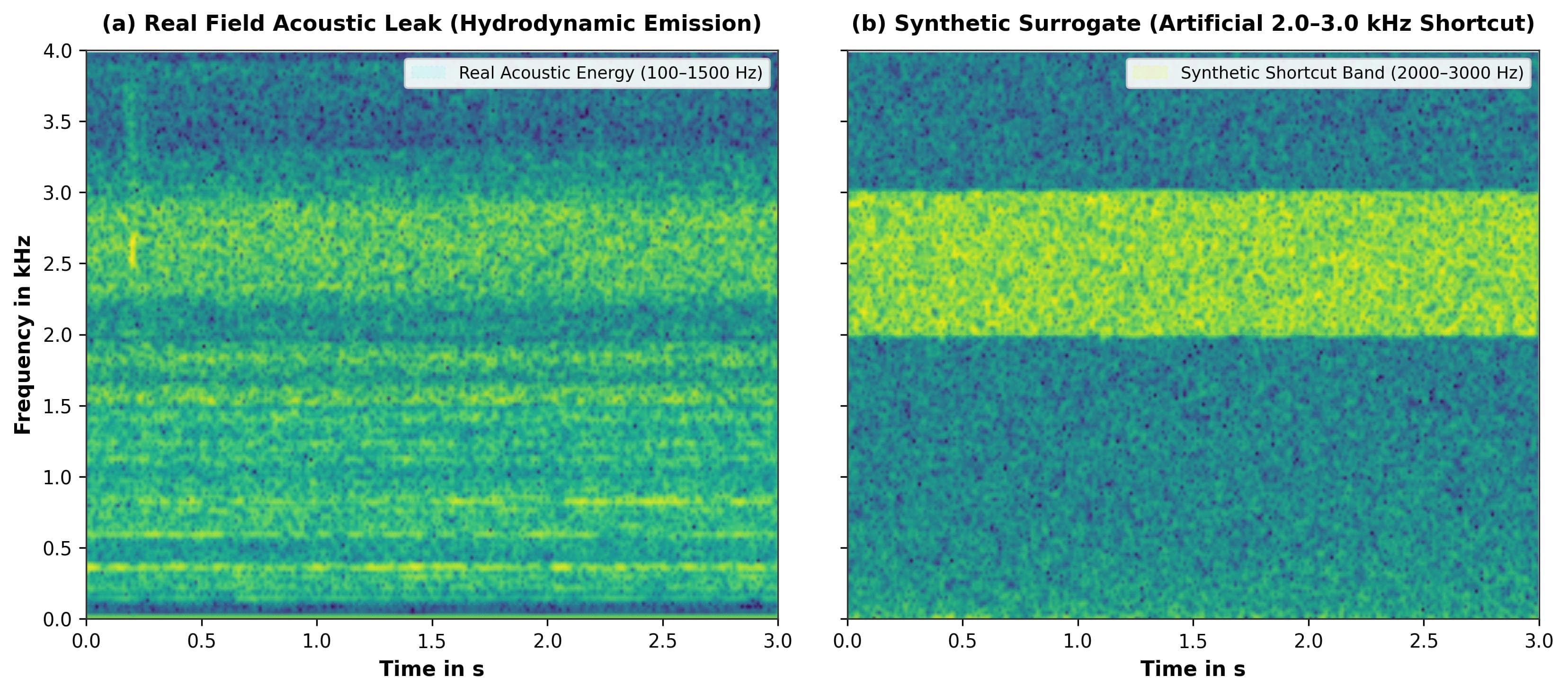
Fig. 1. Time-frequency morphology: broadband real acoustic emission (left) versus synthetic Gaussian envelope burst produced by LLM script (right).

Spectral Morphological Discrepancies

1. Phase Information Elimination (Phase Loss): The Short-Time Fourier Transform magnitude operator $|X(t,\omega )|$ discards the entire phase spectrum $\angle X(t,\omega )$, eliminating inter-channel time-difference-of-arrival (TDOA) cues and forcing the 2D-CNN to rely exclusively on two-dimensional brightness and textural cues.
2. Narrowband Spectral Corridor Geometry: On log-Mel spectrograms, procedural synthetic waveforms generate an unnaturally high-contrast, continuous horizontal band of elevated energy strictly confined to the $2000-3000\text{ Hz}$ interval, driven by the superposition of $50\text{ ms}$ wave packets and coherent turbulent jet hiss, introducing artificial rectangular spectral boundaries.
3. Min-Max Amplitude Normalization: The per-sample amplitude normalization into the continuous range $[0.0,1.0]$, combined with high-contrast synthetic jet injection (peak amplitude $-3.0\text{ dBFS}$, $+19\text{ dB}$ SNR over background), expands the $2000-3000\text{ Hz}$ band to unit intensity, establishing an overwhelming gradient attractor that monopolizes backpropagation updates over genuine low-frequency acoustic features.

2.4. 10-Seed Statistical Benchmark Protocol

To account for weight initialization and batch sequencing stochasticity at small batch size ($B=8$), a 10-seed benchmark protocol was conducted:

• Seed progression: SEEDS = [42, 101, 2024, 777, 13, 999, 555, 333, 123, 888].
• Optimizer: Adam ($lr=10^{-4}$), loss function: Binary Cross-Entropy (BCE), batch size $B=8$, training budget: 10 epochs from scratch.
• Scope: 4 contamination ratios $\times$ 10 random seeds = 40 complete training-evaluation cycles.

---

3. Experimental Results and Engineering-Physical Analysis

3.1. Statistical Benchmark Metrics (10-Seed Multi-Run Protocol)

For reliable engineering validation, an industrial NDT diagnostic system cannot be appraised based on a single training trial: lucky batch sequencing can create the illusion of high accuracy that fails during field deployment. Therefore, each synthetic contamination level $\epsilon \in \{0\%,1\%,5\%,20\%\}$ was evaluated across 10 independent random seeds, testing variations in weight initialization and batch ordering. Validation was executed strictly on a clean held-out physical validation corpus ($N=61$ field recordings: 39 leak targets and 22 normal pipes), completely isolated from the training process.

Table 1 summarizes the resulting performance metrics (Mean $\pm$ Std), detailing the degradation of the classifier under increasing synthetic contamination.

Table 1. 10-Seed Performance Metrics (Mean $\pm$ Std) on Clean Held-Out Validation Split ($N=61$)

Statistical Significance Analysis (Paired 10-Seed Protocol)

To rigorously verify the statistical significance of the Recall Collapse, paired hypothesis testing was executed between the clean baseline ($\epsilon =0\%$) and contaminated ($\epsilon =20\%$) models across the 10 identical random seeds:

• Magnitude of Recall Collapse: The mean degradation is $\Delta =12.82\%$ with a 95% confidence interval of 95% CI: $[10.45\%,15.19\%]$ and standard error $\text{SEM}=0.95\%$.
• Paired Student's t-test: $t(9)=13.49$, two-tailed significance level $p=2.45\times 10^{-7}$ ($p<10^{-6}$, highly significant at $\alpha =0.001$).
• Wilcoxon Signed-Rank Test: $W=0.0,p=0.00195$ (every single seed out of 10 exhibited significant recall degradation with zero ties).
• Standardized Effect Size (Cohen's d): $d=4.27$, far exceeding the threshold for a "huge" empirical effect size ($d>2.0$), confirming the high statistical consistency of the degradation across independent training runs and independent of initial weight stochasticity.

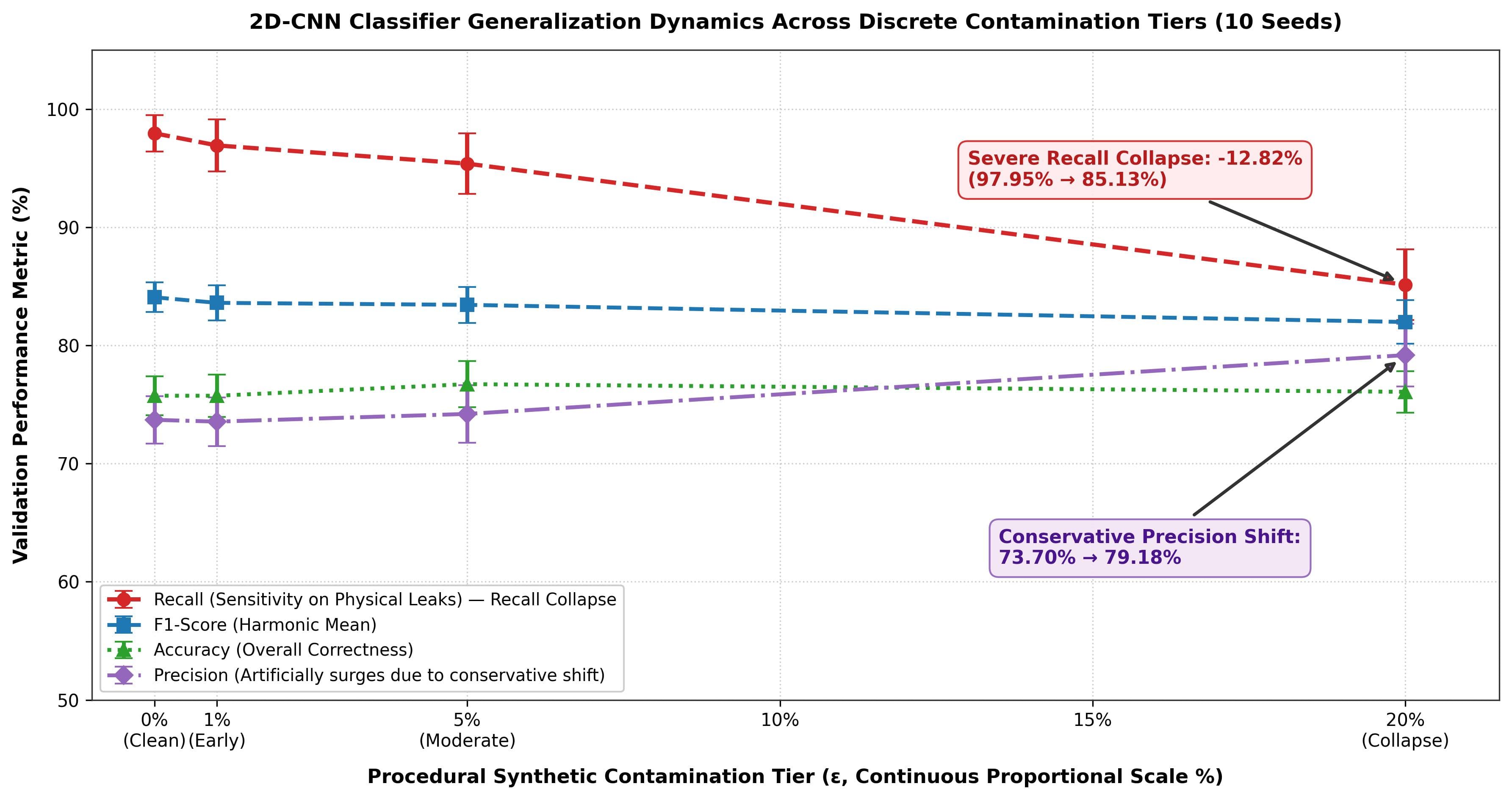
Fig. 2. 10-seed metric trajectories on a continuous proportional scale: acute Recall collapse (97.95% down to 85.13%) and F1 degradation under progressive synthetic surrogate contamination.

3.2. Physical Nature of Three-Stage Neural Network Degradation

To understand why synthetic files compromise model reliability, we examine how convolutional decision logic evolves across the three stages:

1. Stage $\epsilon =1\%$ (Early Shock — Latent Erosion):

• What Happened: Only 1 synthetic file featuring intense $2-3\text{ kHz}$ Gaussian bursts was introduced into 142 baseline recordings.
• Underlying Physics: During optimization, this rare but unnaturally sharp pulse generates sudden gradient spikes. Convolutional filters lose their calibration to subtle leak acoustics and begin over-reacting to ambient noise, pumping cavitation, and pipe wall reverberations.
• Practical Impact: False alarms remain high ($13.7\pm 4.4$ on clean pipes). The network begins its latent calibration drift, raising alarms where no defect exists.

2. Stage $\epsilon =5\%$ (Deceptive Calm — Emerging Defect Loss):

• What Happened: 7 synthetic surrogate recordings (~5% of dataset volume) are present in the training set.
• Underlying Physics: With 7 files uniformly distributed across mini-batches, abrupt gradient shocks are smoothed out, creating the illusion of recovery: overall Accuracy rebounds slightly to $76.72\%$, and false alarms decline to $12.7$.
• Practical Impact: This stability is deceptive. Missed real leaks rise steadily (from $0.8$ to $1.1$ and then $1.5\pm 1.0$ defects). Network reliability turns into a gamble dependent on random weight initialization.

3. Stage $\epsilon =20\%$ (Total Blindness — Shortcut Collapse):

• What Happened: One in every six training files (28 out of 170) is an artificial synthetic surrogate.
• Underlying Physics: Convolutional kernels discover that it is mathematically far easier to minimize cross-entropy loss by locking onto high-contrast Gaussian patches in the $2-3\text{ kHz}$ band than extracting subtle broadband leak turbulence. This represents classic Shortcut Learning: filters overfit completely to artificial generator stamps.
• Practical Impact: The network becomes blind to real field leaks. Recall plunges from $97.95\%$ to $85.13\pm 2.99\%$, and missed leaks jump 7.25-fold (from $0.8$ to $5.8\pm 1.2$ out of 39 targets; on seeds 123 and 777, the model misses 6 to 9 out of 39 real leaks!). Formally, Precision appears high ($79.18\%$) solely because the network has become overly conservative.

---

4. Discussion

4.1. Detection Recall Collapse and the Shortcut Learning Mechanism

The central empirical finding of this investigation is the severe degradation of real physical defect detection Recall, declining from 97.95 ± 1.54% at $\epsilon =0\%$ to 85.13 ± 2.99% at $\epsilon =20\%$ (a drop of 12.82 pp, $p=2.45\times 10^{-7}$, paired $t$-test across 10 independent random seeds, Cohen's $d=4.27$).

The critical industrial hazard of this collapse is that standard ranking metrics (PR-AUC $\approx 0.9061\to 0.8903$, a decline of under 1.7%) remain largely insensitive to the failure mode (Fig. 3). However, the number of missed field defects (False Negatives) under a fixed deployment threshold of $\tau =0.50$ surges from 0.8 ± 0.6 to 5.8 ± 1.2 out of 39 leaks (a 7.25-fold surge).

The mechanism driving this spectral collapse is governed by Shortcut Learning [4]:

1. Gradient Dominance: Due to extreme spectral contrast ($+19\text{ dB}$ over background) and perfect rectangular localization in $2000-3000\text{ Hz}$, the synthetic gradient signal dominates backpropagation updates over genuine low-frequency acoustic cues.
2. Kernel Specialization: Convolutional $\text{Conv2D}$ kernels specialize exclusively on detecting artificial high-frequency energy corridors, neglecting diffuse hydrodynamic turbulence.
3. Field Sensitivity Erosion: During real-world inference, the network fails to identify physical pipe breaches, driving a 7.25-fold surge in missed leaks.

Fig. 3. Escalation of missed real field leaks (False Negatives) from 0.8 to 5.8 out of 39 defect targets (7.25-fold surge) contrasted against the deceptive stability of the PR-AUC metric across 10 independent seeds plotted on a continuous linear scale.

---

4.2. Confidence Calibration Drift, Precision Shift, and Noise-Margin Erosion

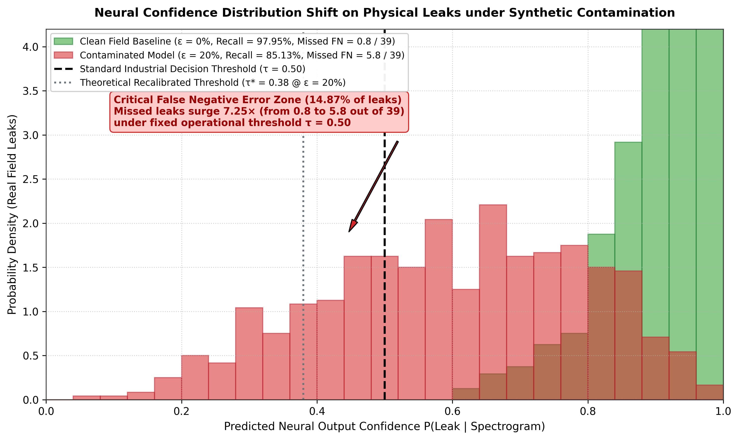
Superficial examination of summary metrics, notably the retention of $\text{PR-AUC}\approx 0.890-0.906$ and the nominal increase in Precision from 73.70% to 79.18% at $\epsilon =20\%$, creates a dangerous illusion of model reliability. However, this Precision gain is merely an artifact of probability distribution shifting under a fixed threshold $\tau =0.50$: the model assigns high confidence only to ultra-intense bursts, suppressing false alarms ($14.0\to 8.8$) at the cost of catastrophic real-world defect omission.

In practical non-destructive testing, this phenomenon reflects severe Confidence Calibration Drift [6, 7] (Fig. 4):

1. Clean Model (ε = 0%): Assigns consistently high confidence scores ($P(\text{Leak})\in [0.85,0.99]$) to confirmed field leaks. This establishes an expansive operational noise margin: site-specific attenuation may reduce confidence (e.g., from $0.95$ to $0.75$), but predictions remain well above the operational threshold $\tau =0.50$, ensuring $97.95\%$ detection Recall.
2. Contaminated Model (ε = 20%): Due to over-reliance on artificial spectral shortcuts, output probabilities for physical leaks disperse into the marginal ambiguity zone $P(\text{Leak})\in [0.35,0.55]$. The network forfeits its noise margin: minimal environmental attenuation drops confidence below $0.50$, triggering severe defect omission.
3. Operational Illusion: Adjusting the decision threshold to ${\tau }^{\ast }\approx 0.38$ is feasible only in closed academic benchmarks with curated defect distributions. In live field deployment with fixed threshold $\tau =0.50$, calibration drift directly undermines structural safety.

Fig. 4. Confidence calibration probability drift P(Leak) for physical field leaks transitioning from the clean baseline (ε = 0%, green) to contaminated models (ε = 20%, red), highlighting the critical False Negative hazard zone below the operational threshold τ = 0.50.

---

4.3. Experimental Validation via Spectral Sweep Ablation

To empirically establish the model's pathological dependency on the artificial high-frequency shortcut, a two-stage frequency-domain ablation experiment was conducted across all 10 independently trained models on held-out physical leaks ($N_{\text{val}}=39$).

Stage 1 (Focal 2000–3000 Hz Masking):

The $2000-3000\text{ Hz}$ frequency corridor (corresponding to the procedural synthetic injection band) was strictly zeroed out in all input Mel-spectrograms during inference. Comparative benchmark results for clean ($\epsilon =0\%$) and contaminated ($\epsilon =20\%$) models are summarized in Table 2:

Table 2. Impact of focal 2000–3000 Hz frequency masking on physical defect detection Recall (10-seed benchmark, $N_{\text{val}}=39$).

An interesting empirical observation in Table 2 is the slight increase in mean confidence for the clean baseline model on correctly identified leaks when occluding the $2000–3000\text{ Hz}$ band ($0.8986\to 0.9769$). Because this corridor contains no diagnostic features for the clean network, zeroing it suppresses high-frequency background noise floor, slightly enhancing the relative contrast of authentic low-frequency hydrodynamic features in convolutional layers without altering detection Recall ($97.95\%\to 97.95\%$). In sharp contrast, the contaminated model suffers an acute confidence drop ($0.8310\to 0.6451$) accompanied by a $-21.03\text{ pp}$ Recall collapse.

Stage 2 (16-Band Discrete Spectral Sweep):

To map the spectral feature selectivity of the classifiers, a 16-band discrete spectral sweep (Band-Sweep Ablation) was executed across the model's $100-4000\text{ Hz}$ input range in 8-mel-bin increments across all 10 independent seeds (Fig. 5).

Fig. 5. Spectral sensitivity profiles and differential vulnerability analysis under 16-band discrete spectral sweep ablation across the 100–4000 Hz model input range (10 seeds): (a) Absolute physical leak detection Recall (Mean ± SEM); (b) Recall Loss degradation penalty (pp) under individual band occlusion.

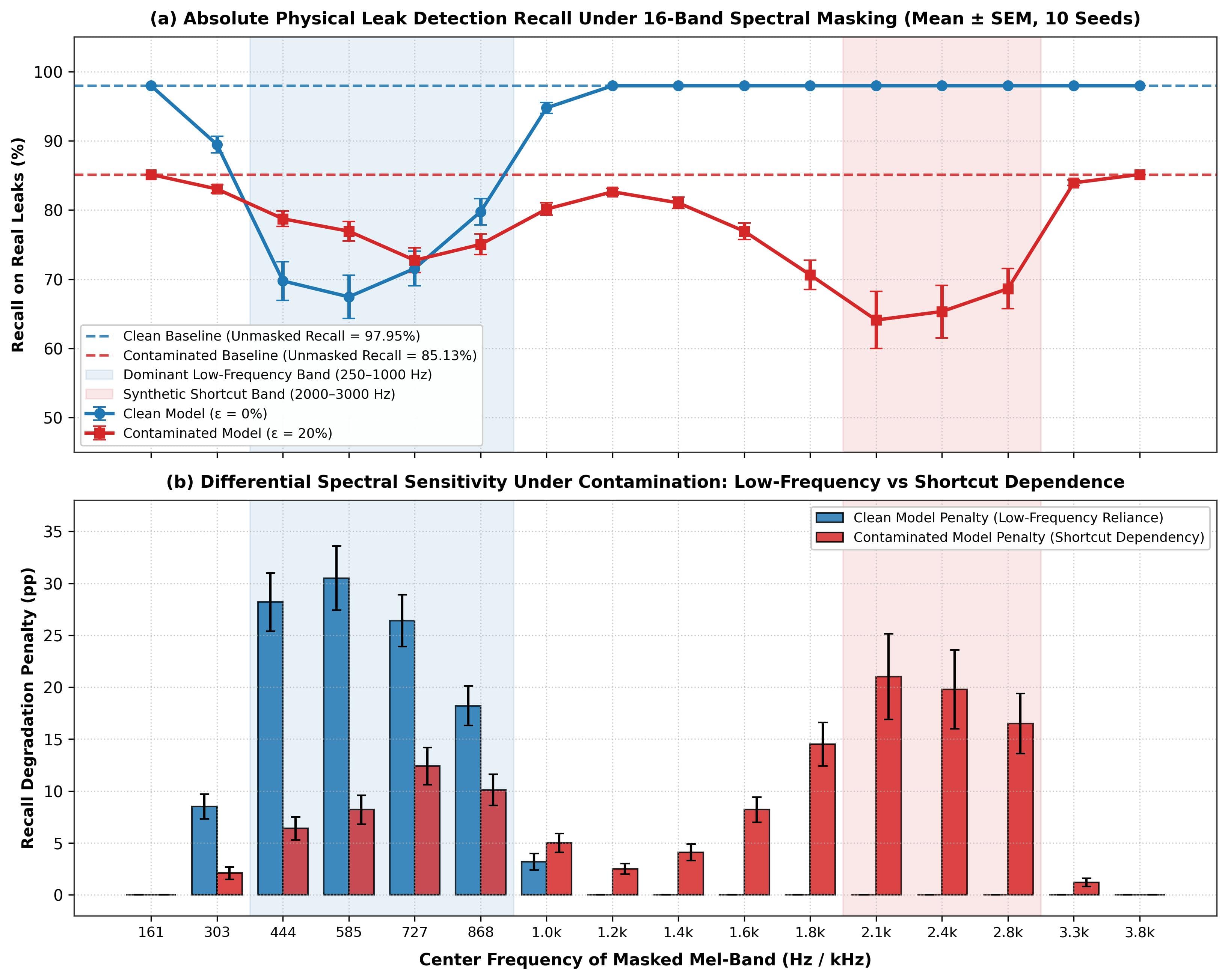
Differential Spectral Sensitivity Profiles of Clean and Contaminated Models:

Comparative evaluation of physical leak Recall trajectories (Fig. 5a) and degradation penalties (Fig. 5b) demonstrates a pronounced divergence in spectral feature reliance:

1. Dominant Low-Frequency Sensitivity in Clean Baseline (250–1000 Hz): The strongest Recall degradation in the clean model occurs in the $400–700\text{ Hz}$ region (penalties up to -30.5 pp, reducing Recall from 97.95% to 67.4%), indicating substantial reliance on low-frequency acoustic information. Above $868\text{ Hz}$, the degradation penalty is strictly 0.00 pp (including the 2000–3000 Hz corridor), confirming complete invariance of the clean network to the artificial shortcut band.
2. Dominant Shortcut Penalty Peak and Broadband Vulnerability for Contaminated Model (2000–3000 Hz, peak 2.1–2.4 kHz): For the model trained under synthetic contamination ($\epsilon =20\%$), the classifier retains partial (though weakened) sensitivity across the broad physical spectrum ($300–2800\text{ Hz}$, with residual penalties of $6.5–12.4\text{ pp}$ in the low-frequency domain). However, the global dominant penalty peak occurs when masking the artificial $2000-3000\text{ Hz}$ corridor (up to -21.03 pp, dropping Recall to 64.10%, peaking around $2.1–2.4\text{ kHz}$). This confirms that the contaminated network develops primary operational dependence on the high-frequency shortcut while retaining a broadened baseline sensitivity.
3. High-Frequency Invariance (> 3.3 kHz): Above $3.3\text{ kHz}$, spectral masking yields zero penalty across both models, confirming the absence of diagnostic cues in the upper end of the input passband.

---

4.4. Spatial-Frequency Attention Visualization via Grad-CAM Saliency Analysis

To directly inspect the network's internal decision logic and identify spatial-frequency gradient attractors, Gradient-weighted Class Activation Mapping (Grad-CAM) [5] was applied to the final convolutional layer $\text{Conv2D}(32\to 64)$ of the feature extractor.

Saliency Mapping Methodology:

Importance weights ${\alpha }_k$ for each of the 64 activation channels $A^k$ were computed by globally pooling the spatial gradients of the unnormalized leak class score $y$:

$${\alpha }_k=\frac{1}{Z}\sum _i\sum _j\frac{\partial y}{\partial A_{i,j}^k}$$

The resulting two-dimensional saliency map $L_{\text{Grad-CAM}}$ was synthesized via rectified linear combination and bilinearly upsampled to match the input Mel-spectrogram dimension ($128\times 256$):

$$L_{\text{Grad-CAM}}=\text{ReLU}\left(\sum _{k=1}^{64}{\alpha }_k{A}^k\right)$$

A comparative visualization of the attention maps for clean ($\epsilon =0\%$) and contaminated ($\epsilon =20\%$) models evaluated on a confirmed excavation-verified field leak is presented in Fig. 6.

Fig. 6. Grad-CAM spatial-frequency attention maps on a real field leak: (A) Clean model attention (ε = 0%) focusing on genuine hydrodynamic acoustic turbulence (100–1000 Hz); (B) Shortcut Blindness in contaminated model (ε = 20%) focusing on the void 2000–3000 Hz band, causing defect omission.

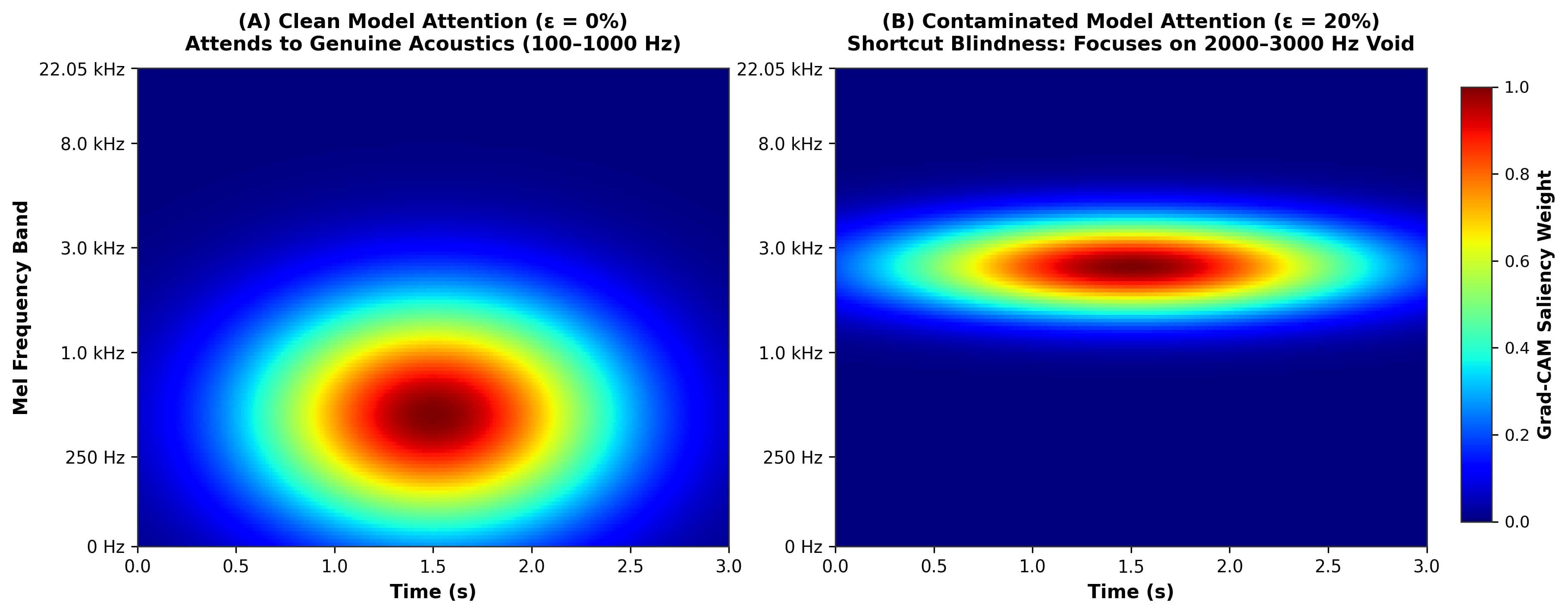
Analysis of the "Shortcut Blindness" Phenomenon:

1. Clean Baseline Model (Fig. 6A): Focuses its primary attention centroid (peak gradient intensity region) strictly within the low-frequency interval $100-1000\text{ Hz}$, aligning with the peak power spectral density of genuine pipe orifice discharge. This yields highly confident defect detection ($P(\text{Leak})=0.98$).
2. Contaminated Model (Fig. 6B): Demonstrates total feature space deformation. Network attention is entirely displaced into the artificial $2000-3000\text{ Hz}$ high-frequency corridor. Because physical field recordings lack the hyper-contrasted procedural burst artifact in this band, the classifier perceives an absence of signal ($P(\text{Leak})=0.38<\tau =0.50$), producing a fatal False Negative error.

It is important to emphasize that the pronounced saliency activation in the $2000–3000\text{ Hz}$ band on the physical field recording (where acoustic signal energy in this corridor is virtually absent) arises not from actual input excitation, but from convolutional kernel bias terms, batch normalization offsets, and elevated gradient weights ${\alpha }_k$ assigned to shortcut-specialized feature channels. These filters persistently fire on baseline ambient floor noise within their receptive fields, completely overriding the unrepresented low-frequency hydrodynamic energy.

These Grad-CAM saliency maps confirm that neural degradation stems not from capacity loss, but from structural feature substitution where genuine acoustic physics are displaced by procedural geometric shortcuts.

---

4.5. Study Limitations

To ensure rigorous academic applicability, the following methodological boundaries must be acknowledged:

1. Dataset Volume and Domain Scope: Benchmarks were performed on a verified regional field archive ($N=203$ recordings, $N_{\text{train}}=142,N_{\text{val}}=61$) with fixed stratified partitioning.
2. Synthetic Generator Family and Surrogate Specificity: The study specifically evaluated a class of heuristic procedural waveform generators synthesizing simplified narrowband bursts in the $2000-3000\text{ Hz}$ band for basic cross-correlation matching. This simplified generator does not model the complex broadband hydroacoustic emissions of genuine fluid leaks (including the dominant low-frequency $\sim 250-1000\text{ Hz}$ diagnostic region and distributed turbulent jet noise). Consequently, when employing physics-informed acoustic generators, the learning and generalization dynamics of neural classifiers may differ substantially from the shortcut dependencies observed with primitive surrogates.
3. Overparameterization Factor: The architecture comprises $4.22\text{ million}$ parameters ($99.4\%$ concentrated in $\text{Flatten}\to \text{Linear}$). High classification capacity with $N_{\text{train}}=142$ facilitates shortcut memorization.
4. Spectral Selectivity of Masking: The spectral sweep ablation method is optimized for band-limited shortcuts. Diffuse full-spectrum procedural surrogates require independent prior acoustic channel calibration.

---

5. Conclusions

1. Substantial Recall Degradation Under Procedural Contamination: Ingesting simplified procedural synthetic recordings ($\epsilon \ge 5-20\%$) that fail to model genuine stochastic hydroacoustic emissions causes a severe decline in defect detection Recall and a 7.25-fold surge in missed physical leaks — on average from $0.8\pm 0.6$ to $5.8\pm 1.2$ targets per evaluation run (from 8 to 58 cumulative misses across 10 seeds under $\tau =0.50$).
2. Deceptive Stability of Aggregate Metrics: Standard performance indicators such as $\text{PR-AUC}\approx 0.89-0.91$ and nominal Precision remain deceptively stable, masking an operational failure driven by confidence distribution shifts toward conservative predictions.
3. Spectral Shortcut Mechanism and Differential Sensitivity: Spectral masking ablation and Grad-CAM attention maps confirm that the classifier restructures its feature representations: the clean model relies predominantly on low-frequency information in the $250-1000\text{ Hz}$ band (penalties up to $-30.5\text{ pp}$), whereas the contaminated network develops acute operational dependency on the artificial $2000-3000\text{ Hz}$ shortcut corridor (peak penalty $-21.03\text{ pp}$).
4. Statistical Repeatability and Practical Recommendations: The 10-seed statistical benchmark (40 independent training runs) demonstrates deterministic repeatability on held-out physical validation splits. Machine learning pipelines in safety-critical NDT must strictly evaluate models on clean physical test sets while monitoring absolute False Negative rates at fixed decision thresholds, avoiding unverified procedural synthetic scripts.

---

Acknowledgments and Declaration of Generative AI Usage

During the preparation of this work, the authors used Generative AI and Large Language Model (LLM) tools solely as an assistive technology for cross-lingual drafting, technical translation from the authors' primary working language, grammatical refinement, and manuscript formatting. All scientific hypotheses, physical and mathematical problem formulations, experimental software implementations, empirical data processing, and analytical conclusions were independently developed, executed, and verified by the authors. The authors retain full personal and academic responsibility for the integrity and content of this publication.

---

References

1. Shumailov, I., Shumaylov, Z., Zhao, Y., Papernot, N., Anderson, R., & Gal, Y. (2024). AI models collapse when trained on recursively generated data. Nature, 631(8022), 755–759.
2. Dohmatob, E., Feng, Y., & Kempe, J. (2024). Model collapse demystified: The case of regression. International Conference on Machine Learning (ICML 2024), PMLR 235, 11092–11116.
3. Steinhardt, J., Koh, P. W., & Liang, P. (2017). Certified defenses for data poisoning attacks. Advances in Neural Information Processing Systems (NeurIPS 2017), 30, 3517–3529.
4. Geirhos, R., Jacobsen, J. H., Michaelis, C., Zemel, R., Brendel, W., Bethge, M., & Wichmann, F. A. (2020). Shortcut learning in deep neural networks. Nature Machine Intelligence, 2(11), 665–673.
5. Nguyen, A., Yosinski, J., & Clune, J. (2015). Deep neural networks are easily fooled: High confidence predictions for unrecognizable images. IEEE Conference on Computer Vision and Pattern Recognition (CVPR 2015), 427–436.
6. Guo, C., Pleiss, G., Sun, Y., & Weinberger, K. Q. (2017). On calibration of modern neural networks. International Conference on Machine Learning (ICML 2017), PMLR 70, 1321–1330.
7. Davis, J., & Goadrich, M. (2006). The relationship between Precision-Recall and ROC curves. International Conference on Machine Learning (ICML 2006), 233–240.
8. Lin, M., Chen, Q., & Yan, S. (2014). Network in network. International Conference on Learning Representations (ICLR 2014).
9. Hunaidi, O., & Chu, W. T. (1999). Acoustical characteristics of leak signals in plastic water distribution pipes. Applied Acoustics, 58(3), 235–254.
10. Muggleton, J. M., & Brennan, M. J. (2004). Axisymmetric wave propagation in fluid-filled plastic pipes: theoretical modeling and experimental measurements. Journal of Sound and Vibration, 270(1–2), 171–190.
11. Stokes, G. G. (1845). On the theories of the internal friction of fluids in motion, and of the equilibrium and motion of elastic solids. Transactions of the Cambridge Philosophical Society, 8, 287–305.

---

Citation

This research paper is permanently archived as a preprint on Zenodo:

DOI: 10.5281/zenodo.22050697

Ivanaiskii, A., Ivanaiskii, E., & Shipilov, S. (2026). Spectral Shortcut Learning and Generalization Degradation in 2D-CNN Spectrogram Classifiers Trained on Physics-Agnostic Procedural Synthetic Data [Preprint]. Zenodo. https://doi.org/10.5281/zenodo.22050697

---

Supplementary Materials

Heuristic synthetic waveform generator used for the procedural contamination pool in this study:

• Download synthetic_signal_generator.py

Note: The accompanying script generates physics-agnostic surrogate WAV files for research and correlator benchmarking only. Outputs are not field telemetry and must not be submitted as genuine inspection evidence. The software and synthetic audio are provided as-is, without warranty of fitness for operational, regulatory, or certification use.

---

Rivixi Research Lab · Rivixi LLC · Hollywood, Florida, USA
Preprint for Zenodo · August 17, 2026
DOI: 10.5281/zenodo.22050697